Chapter 4
CRAFTING ECONOMIC DRIVERS FOR SUSTAINABLE LOCAL AREAS IN A GLOBALISING REGIONAL ECONOMY: SYDNEY AS A CASE STUDY
Sydney is facing its future. It is the largest city and one of the fastest growing metropolitan areas of Australia. Like many newly emerging global cities, Sydney is dealing with its past economy while it shapes its future economic scenarios. Spatially uneven outcomes seem inevitable as metropolitan regions globalise. But for Sydney, this transition is especially painful when the nation bases its sociopolitical fabric on equal outcomes – ‘a fair go’ for all citizens. In response to change, Sydney has adopted a new approach to metropolitan planning that has moved from a traditional land use system to one that comes to grips with socioeconomic issues.
Using tools of small area analysis of the internal spatial economies of the Sydney metropolitan region, this chapter looks at how the region could reach new strategic goals with a more equitable metropolitan economic pattern. The analytical template for this approach is a new form of metropolitan suburban district analysis of a greater metropolitan system. This research uses city/suburban data to explore patterns of spatial drivers in the metropolitan system. These are tracked internally their implications for the performance of a regional spatial economy are assessed. The research offers explanations and a mechanism to identify the causes and consequences of unequal metropolitan economic performance. Furthermore, it provides an alternative for crafting economic drivers for sustainable local area development in a globalising regional economy in a more equitable and stronger performing region. 71
Introduction
One of the more troubling aspects of the new global regional economics is spatial inequality (Goldsmith and Blakely, 1992). In crafting a future economic scenario for a large globalised region, there are locational winners and losers. For decades, central city and older suburban areas have declined in the wake of globalisation. This process of unevenness is now a central issue in regional plan making (Hill and Wolman, 1997; Ledebur and Barnes, 1992). The reason for this fascination with unequal subregional development can be traced to studies of US inequalities between central cities and the growing suburban areas. Much of the US work in regional economic inequality reflects the racial and spatial outcomes of metropolitan areas (Kasarda and Parnell, 1993), the latter represented as a spatial economic apartheid and the central thesis of recent American regional scholarship. Douglas Massey and Nancy Denton’s classic work, American apartheid: segregation and the making of the American underclass (1993) details the deep division of resources between haves and have-nots occupying the same regional economic geography.
But space and race are not the only reasons for differential economic outcomes between suburbs and central cities in the United States. Myron Orfield (1997) provides a different analysis of the regional suburbanised economy in the Minneapolis-St. Paul region to show how underlying policy and economic migration factors undermine city economies and generate suburban advantages as a region globalises creating inter and intra-city disparities (p. 67). The consequences, as Orfield (1997) has noted are sprawl and uneven wealth distribution among suburbs. Essentially, the new economy is not just about suburbs and the inner city but also and most importantly about the specific economies of suburbs and specific parts of the inner city.
Moreover, in some parts of the world, including Sydney, it is the outer suburbs, rather than the central city, where emerging inequality is pronounced and more deeply embedded in the socioeconomic structure. While race may be a prime factor for unequal allocations in the US, this is not the case in Sydney where recent immigration patterns and other factors, as is the case in many European cities, are at work that create uneven spatial economies. Michael Stoll (1999), a researcher specialising in poverty, race and space, suggests that being near work does not guarantee that residents in a global region are able to gain work 72irrespective of race. As this research shows, spatial economic drivers in different parts of a region can have profound effects on the nature and course of globalisation. This chapter looks at uneven regional performance in Sydney, Australia to find the economic drivers that generate economic disparities across a region. It suggests the keys to intervening that might help make underperforming places more competitive as the region’s economy is transformed by global economic forces. Sydney is an ideal case of spatial redistributions as a result of international forces since it is isolated from border incursions or easy access by migrants and has a long history of national economic management aimed at even distribution of wealth (Stimson et al., 2002).
Sydney metropolitan region
The Sydney economy has grown for the last three decades adding jobs and people. Sydney grew 707,075 jobs over 25 years and increased its population by 1,113,601 over the same period ― a ratio of 0.63. Sydney is the largest recipient of international immigration and internal emigration within the nation. The new immigrant human resources added to Sydney are an economic dimension since many come with high skills or come seeking tertiary education opportunities and remain in Sydney adding to the regional skill pool, which attracts new firms and enhances existing firms’ competitiveness (O’Connor, 1999).
Sydney is undergoing a new metropolitan regional strategic planning process (Searle, 1996). Unlike former regional plans that focused almost solely on allocating land for housing estates, this puts a greater emphasis on using tools to affect spatial economic outcomes. The new Sydney Strategic Plan is designed to influence spatial allocation of job creation opportunities and to improve spatial economic wellbeing across the entire metropolitan area (DIPNR, 2005). Sydney is not alone in seeking to use planning tools for a more just socioeconomic outcome. The new London Plan has the same goals with only a slightly different emphasis. Similar ideas are expressed in regional plans for Long Island in New York, Seattle, San Francisco and Paris. The theme of spatial inequality is central to regional science. However, most regional science tools are aimed at addressing smaller grained problems in the regional economic network for Sydney or other similar regions. 73
Sydney and Australia are characterised as a homogenous national spatial economy. For over half a century, Australian wages have been set through national wager tribunals and working conditions organised to present uniform entitlements. Moreover, public investments such as schools, roads and the like have been more evenly provided through state institutions. Yet as Sydney embarks on its fourth major metropolitan plan the central issue is job and income fragmentation. In essence, Sydney and Australia have joined the global market place. Despite more even public infrastructure endowments, Sydney is becoming increasingly economically segregated with different economic drivers altering the socioeconomic outcomes across the region. In this research we look for the subregional drivers of local city jurisdictional areas as micro-regional spaces vs. the macro-region of Sydney’s metropolitan system of nearly 5 million people to see how regional science can help identify and correct the gaps in regional economic outcomes as the region and the nation globalise. Unless the pattern of local economic drivers in spatial areas below the large metro-region are understood, it is difficult to apply spatially sensitive actions through planning schemes that generate more equal outcomes for areas that are socially and spatially disadvantaged by the globalisation processes. We do not have the space to present the history of Sydney’s economy here but there is substantial data on how spatial inequalities arose over time (Searle, 1996). We therefore focus on spatial economic drivers across the Sydney region through the lens of city jurisdictional nodes to provide better guidance for local suburban and regional policymakers as they craft regional economic policies.
Study scope
This study uses regional economic analysis tools to look at the structure of Sydney’s subregions or districts (Illawarra, Hunter, Western Sydney etc.), the statistical local areas that cover the Sydney Greater Metropolitan Region (GMR) (see Figure 16). It undertakes a comprehensive analysis using income and population growth as proxies for socioeconomic prosperity in the localities studied. We select these key variables because in combination they illustrate socioeconomic health. While population loss can be an indicator in a mature economy of community decline, rising incomes are a strong measure of wealth. However, there are circumstances where these variables might be false 74signals. For example, an old community might have high incomes but is ageing with a declining population. Or, a fast growing place with new lower socioeconomic immigrant residents might seem like it is doing well, but the human resources and skill levels base might not produce a strong economy despite apparent population growth. Therefore, in this study, we look at population and income from various analytical perspectives to determine the drivers of growth and the decline in the statistical local jurisdiction and aggregated subregional districts of the economy of the Sydney GMR as a whole. Statistical Local Areas (SLAs), which are city sized jurisdictional areas, were used as the basis of the analysis. We note that regional areas the size of US style Standard Metropolitan Statistical Areas (SMSAs) are convenient for firm based economic analysis, but fail to reveal the difference in social demographic spatial outcomes at a lower city sized level. For example, while Orange County or Long Island may look at wealth in aggregate, there are well known pockets of poverty lying in the larger spatial system. In this work, we look at the differential drivers at the micro-city spaces of fast growing economies in a robust region to see where and why differential patterns emerge and what might be done about them. An essential question is: do some places perform better or worse than their neighbours in the same economic space? If so, what are the economic drivers for these divergences in performance?
This research uses Australian Bureau of Statistics (ABS) data for 1990–2001, data sets developed by the Bureau of Transport and Regional Economics (BTRE, 2003b, 2004 and 2005), and specific ABS data for the local areas. Much of the data are four years old, and in a rapidly changing dynamic economy, it may be a better illustration of past performance than an indicator of future directions or barriers. However, it is the best data available and the trend lines are clear and deepening.
Research approach
In this study, we base our examination of the smallest unit for analysis on the statistical local area (SLA), an ABS geographic collection approximating suburbs or closely related groups of small city-suburbs. Our fine grain analysis based on SLAs is richer than is possible in most regions in the United States, where the data available for counties or larger units mask more finely grained spatial differences. 75
SLAs are small and imperfect proxies for subregional economies. We group the statistical local areas in the Sydney GMR into nine natural economic units or districts. These districts are: East Central Sydney, West Central Sydney, North Sydney, South Sydney, North West Sydney, South West Sydney, Illawarra, Newcastle, and Central Coast. Some of these districts remain known for their old economic base while others are clearly influenced by new information industries and new technology. So we look at SLAs across the larger Sydney GMR to see what the drivers of growth are.
Figure 16: Districts in the Sydney Greater Metropolitan Region
| District | Name of Statistical Local Areas Covered | |
| 1 | Eastern Core | Ashfield, Burwood, Canterbury, Concord, Drummoyne, Leichhardt, Marrickville, Strathfield, Botany Bay, Randwick, South Sydney, Sydney Inner, Sydney Remainder, Waverley, Woollahra, Ryde, Hunters Hill, Lane Cove, Mosman, North Sydney, Willoughby (N=21) |
| 2 | Western Core | Auburn, Bankstown, Fairfield, Holroyd, Parramatta (N=5) |
| 3 | North | Hornsby, Ku-ring-gai, Manly, Pittwater, Warringah (N=4) |
| 4 | South | Hurstville, Kogarah, Rockdale, Sutherland E, Sutherland W (N=4) |
| 5 | Northwest | Baulkham Hills, Blacktown – North, Blacktown – SE, Blacktown – SW, Blue Mountains, Hawkesbury, Penrith (N=5) |
| 6 | Southwest | Camden, Campbelltown, Liverpool, Wollondilly (N=4) |
| 7 | Central Coast | Gosford, Wyong (N=2) |
| 8 | Illawarra | Kiama, Shellharbour, Wollongong (N=3) |
| 9 | Newcastle | Cessnock, Lake Macquarie, Maitland, Newcastle – inner, Newcastle – remainder, Port Stephens (N=6) |
| Total | (N =54) |
Source: Authors 76
Analytical methods
The analytical framework of this chapter examines two variables to ascertain regional economic growth – total population and aggregate taxable income. It assesses the drivers or forces that produce either or both. The target or dependent variables are growth in total population (human resources) and growth in aggregate taxable income. These two variables were selected because in combination they are a measure of socioeconomic health. Changes in population size of an area are often associated with changes in a region’s economic activity. In the past, because of a lack of better indicators, population change has often been used as an indicator of regional growth. Rising incomes in a region are strongly related to rising wealth. Nonetheless, there are circumstances where these variables might give false signals because of the rapid growth of new immigrants, lower skilled people, or low income retirees on fixed incomes who relocate to less expensive housing environments such as mobile home parks in Sunbelt areas.
The analysis of this research is threefold. First, location quotients are used to measure the performance of each statistical local area. Location quotients are ideal for ascertaining the performance of places and variables over the same period and using the same base. However, they measure the outcomes, not the inputs that generate relative performance. So, the second stage examines key economic growth activities using economic base analysis methods and correlation analysis. These methods show the relationships between factors associated with economic growth in a SLA to determine which of these factors are significant. Finally, the third stage takes the results of the first two measures and filters them through regressions (multivariate analysis) to see the influences of the significant economic drivers spatially within SLAs in the Sydney GMR. This analytical approach is similar to the work done by Toft and Stough (1986), who look at economic spatial shifts and use shift share with location quotients to measure the rates of growth among regions by comparing regional competitiveness in selected industries (Stimson et al., 2002: p. 87). A similar strategy to that in Stimson et al. (2002) was used in Blakely (1994: p. 113) to establish economic development pathways in the subregions of the Brisbane/Southeast Queensland economy. The analytical approach is outlined in Figure 17. 77
Figure 17: Approach to determining regional economic growth
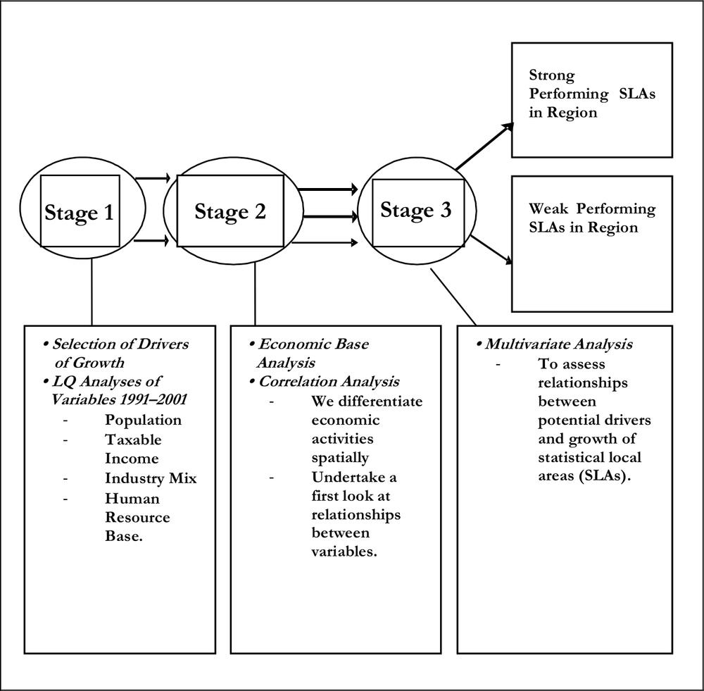
Source: Authors
Location analysis and results
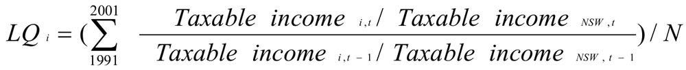
The locational analysis technique is applied to the following variables: population in a region, taxable income in a region, and employment in industries located in the SLAs in the Sydney GMR. This technique was employed to identify the change in selected variables for SLAs between 1991 and 2001. We use the state of NSW as the reference region as has been done in earlier studies (for example, Stimson et al., 2002). The location quotient contains a notion of competition by considering a 78location’s share of the NSW population. The location quotient is used in the same manner as Mikelbank (2005) did to assess the performance of suburbs in the United States. In the case of population for a SLA, the location quotient (LQ) of population for SLA i, is calculated as:

where N denote number of years in the study period. The top term (the numerator) in the equation for population location quotients represents SLA i’s share in the NSW population in time period t. The bottom term (the denominator) in the equation for population location quotients represents SLA i’s share in the NSW population in time period t-1. Thus, any SLA with a population LQ>1 increased its population share over the period. Conversely, a population LQ<1 indicates a decline in that SLA’s NSW population share.
The population location quotients with New South Wales as a reference region show whether a given region grew faster than the overall NSW population (i.e. its LQ>1) or slower than the overall NSW population (i.e. its LQ<1). The LQ analyses, taking the 1991 and the 2001 population, shows that out of 54 SLAs, 24 had LQ values greater than 1, as shown in Figure 18 below. This indicates that the statistical local areas in the following districts – namely, North West of Sydney, South West of Sydney, the Central Coast and the Illawarra regions (i.e. the urban fringe) – stand out as attracting population. On the other hand, the Eastern core of Sydney, the Western core, North and South Sydney (referred to as the global arc) all have at least two-thirds of their statistical local areas with LQ>1. Over the period covered by this study, the global arc lost population share. 79
Figure 18: SLAs with high population location quotient, 1991–2001
| District Name | Number of SLAs with LQ>1 | % of SLAs in the district which have Population LQ>1 | Name of the SLA | Total SLAs in the Districts |
| Eastern Core | 11 | 52% | Botany Bay, Burwood, Concord, Hunters Hill, Lane Cove, Mosman, Strathfield, Sydney Inner, Sydney Remainder, North Sydney, Woollahra | 21 |
| Western Core | 2 | 40% | Auburn, Bankstown | 5 |
| North | 1 | 25% | Hornsby | 4 |
| South | 0 | 0% | 4 | |
| North West | 1 | 20% | Hawkesbury | 5 |
| South West | 3 | 75% | Camden, Liverpool, Wollondilly | 4 |
| Central Coast | 2 | 100% | Gosford, Wyong | 2 |
| Illawarra | 1 | 33% | Kiama | 3 |
| Newcastle | 3 | 50% | Cessnock, Maitland, Newcastle Inner | 6 |
| Total | 24 | 44% | 54 |
Source: Derived by the Planning Research Centre, the University of Sydney and BTRE based on an analysis of Australian Bureau of Statistics Estimated Resident Population, 1991–2001 80
Location quotients – taxable income
Income is a mark of economic strength. The Bureau of Transport and Regional Economics (BTRE, 2005) has argued that aggregate real taxable income in an area can serve as a proxy not only for wealth but also productivity. We look at taxable income changes over the study decade 1991–2001. To generate the results for location quotient analysis of aggregate taxable income for statistical local areas in the Sydney GMR, we used the following equation:
The interpretations of the results for taxable income are similar to those for population. The taxable income location quotients with NSW as a reference region show whether a given SLA’s taxable income grew faster than NSW (i.e., LQ>1) or slower than NSW (i.e., LQ<1). There is a relationship between places that had population growth and those with income growth as shown in Figure 19. The statistical local areas in the Eastern core of Sydney and in North Sydney perform more strongly with respect to income than they do for population. In contrast, statistical local areas on the Central Coast, the Illawarra, and the Southwest of Sydney do well with regard to both population and income growth.
Employment specialisation
This research employed an additional level of analysis to ascertain what industries had impacts on local and subregional economic areas. The data used to determine employment specialisation by statistical local area is from the ABS Census Journey to Work data. Information about journey to work has been collected from the Australian Census of Population and Housing since 1971 (Robertson, 2000). Klosterman et al. (1993) proposed a technique which we use in this section to further look at the statistical local areas by dividing employment in selected industries into two categories: basic and non-basic sector jobs. This technique will enable the identification of which sectors in a statistical local area serve the local market, and which sectors serve a national or international market. The non-local employment is also referred to as basic 81employment. The results from the application of this technique for the statistical local areas in the Sydney GMR are as follows. For each statistical local area, a positive entry indicates the number of non-local jobs in the statistical local areas. A negative entry shows that for that industry, there are no basic (i.e. non-local) jobs in the area.
Figure 19: SLAs with high taxable income quotient, 1991–2001
| District Name | Number of SLAs with LQ>1 | % of SLAs in the district with taxable income LQ>1 | Name of the SLAs |
| Eastern Core | 11 | 67% | Leichhardt, South Sydney, Sydney Inner, Sydney Remainder, Randwick, Waverley, Woollahra, Concord, Drummoyne, Hunter’s Hill, Lane Cove, Mosman, North Sydney, Willoughby |
| Western Core | 2 | 0% | - |
| North | 1 | 100% | Hornsby, Ku-ring-gai, Manly, Pittwater/ Warringah |
| South | 0 | 25% | Sutherland Shire |
| North West | 1 | 60% | Baulkham Hills, Blacktown, Hawkesbury |
| South West | 3 | 75% | Camden, Wollondilly, Liverpool |
| Central Coast | 2 | 100% | Gosford, Wyong |
| Illawarra | 1 | 67% | Kiama, Shellharbour |
| Newcastle | 3 | 17% | Newcastle Inner |
| Total | 24 | 44% |
Source: Derived by the Planning Research Centre, the University of Sydney and BTRE based on analysis of aggregate SLA taxable income, 1990–1 to 2000–1 from Bureau of Transport & Regional Economics (2005) 82
Strengthening and growing the local economy is often related to enhancing the basic sector employment. It also assumes that the basic sector is the engine for the growth of local economies (Klosterman, 1990: p. 115). The employment location quotient (ELQ) of employment for SLA i is calculated as:
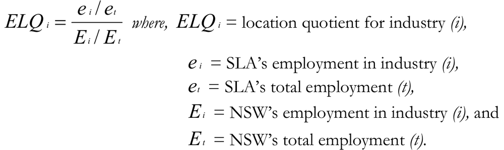
The above tool was employed to identify which industries each district/SLA specialised in, as against the reference region (NSW). The technique measures the extent to which the study district or SLA is specialised relative to the reference region (Klosterman, 1990: p. 129).
If for a given industry, for example manufacturing, the ELQ is greater than one for a SLA, the share of people employed in manufacturing jobs in that SLA’s total employment is larger than the share of NSW people employed in manufacturing jobs in NSW’s total employment. If employment in manufacturing is more important than it is (on average) for the state of New South Wales, the SLA is considered to specialise in manufacturing. Manufacturing for this SLA would be a non-local sector. The SLA would be a net-exporter (to other SLAs) of manufacturing jobs. That is, the supply of manufacturing jobs in the SLA is likely to exceed the demand (capacity to fill) for such jobs in the SLA.
Similarly, if for a given industry the ELQ is less than 1 for a SLA, this means the share of manufacturing jobs in an area’s total employment is less than the share of total employment in NSW manufacturing jobs. This therefore indicates that manufacturing sector jobs are less important in that SLA compared to NSW and that SLA would be a net-importer (from other SLAs) of manufacturing products. Results from the employment specialisation analysis show that in Sydney, the retail sector is performing better than retailing in NSW as a whole. However, the ELQ for the retailing sector is for 19 regions (out of 54) less than 1. 83
From this analysis the anchors of Sydney’s economy are finance, trade and knowledge sector jobs. Sydney’s Western SLAs are home to manufacturing jobs, while Sydney’s South looks like a ‘construction industry’ core, and Newcastle is specialising in health related jobs.
Multivariate analysis of potential drivers of growth
Growth in population and aggregate taxable income
Sydney’s population is growing with most of the GMR’s growth being from natural increase. The remainder comes from Sydney’s attractiveness to people from other parts of Australia and overseas. Population forecasts suggest that about half a million new jobs will be needed over the next 25 years to meet the demands of the ever growing population.
Based on taxable income, the ten fastest growing statistical local areas in the period 1990 to 2001 were: Sydney Remainder, Sydney Inner, Camden, Hunter’s Hill, Mosman, Blacktown, South Sydney, Liverpool, Woollahra, and Leichhardt. Three out of the 10 SLAs with the fastest growth in taxable income are outer fringe SLAs. These are Blacktown, Camden and Liverpool.
However, based on resident population, the ten fastest growing regions in the period from 1991 to 2001 are: Newcastle Inner, Kiama, Sydney Remainder, Sydney Inner, Mosman, Cessnock, Concord, Auburn, Hawkesbury and Maitland. One possible explanation for the fast growth in outer/fringe areas of the Sydney GMR is the high prices of houses in areas closer to the Sydney commercial business district (CBD).
Explanatory variables: factors affecting population growth
The previous section identified the independent or explained variable. This section discusses factors that previous empirical and/or theoretical studies have identified to affect growth of an area. The aim is to identify factors or variables that are associated with growth of total population and/or of aggregate taxable income in a statistical local area. These explanatory variables fall into the following main groups: socioeconomic variables, proxies for human capital in a statistical local area, and industry related variables. These are discussed below. 84
Socioeconomic variables
The regional research literature suggests that the size of a region influences regional growth in two diametrically opposite ways (see for example, Bradley and Gans, 1998). First, regions with a large population may grow slower because of diseconomies of regional size. A region with a large population tends to experience rising housing costs and commuting costs. These factors exacerbate socioeconomic differences across the region and may lead to perceived changes in quality of life in a region and may contribute to lower growth rates. On the other hand, regions with large populations can grow faster because of agglomeration effects (Feser, 2001) including productivity because of a larger labour pool, and because of inter-industry knowledge spill overs between co-located industries which can lead to product variety and diversity and an overall better quality of life.
The justification for including a SLA’s initial period income per taxpayer amongst explanatory variables of growth can be found in the Bureau of Transport and Regional Economics (2005). The research expects a similar negative relationship between income per taxpayer in 1991 and growth in the Sydney GMR from 1991 and 2001.
The Australian Bureau of Statistics (2002) suggests that there may be a relationship between the population density and the population growth of an area. This research hypothesises that population growth will be higher in statistical local areas which in 1991 had lower population densities.
SLA’s human capital
Recent international studies (OECD, 2001a, b, c) of the role of education in relation to skills and qualifications in regional economic performance suggest that human capital has a favourable impact. In this study, we also explore the relationship between the growth of a statistical local area and the following proxies for human capital in a SLA: (a) the percentage of a SLA’s population who had a degree or higher (Ed1) in 1991; and (b) the percentage of a SLA’s population who have completed skilled vocational training (Ed3) in 1991. In this study two variables are used as proxies for a SLA’s human capital. They are: Ed1 – the share of a region’s population with a Bachelor’s degree or higher, and Ed3 – the 85share of a SLA’s population who have a skilled vocational qualification. Exploratory analyses ruled out the use of other possible proxies (which were often insignificant).
Industry-related variables in a SLA
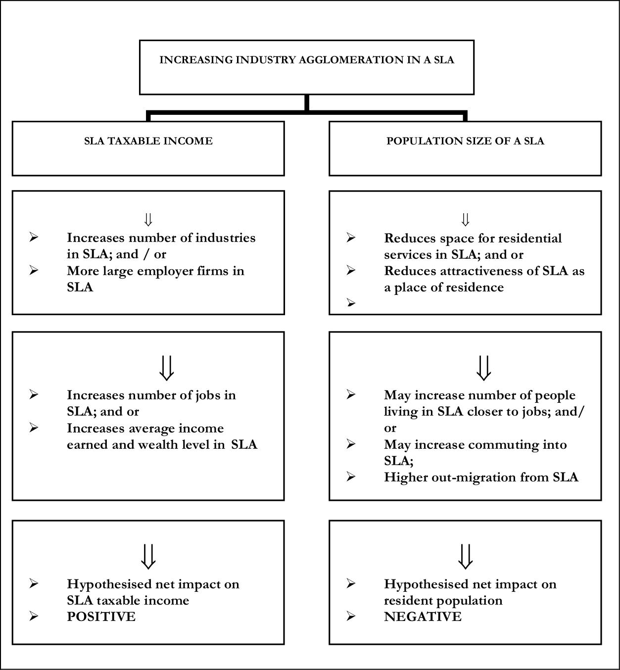
Various theoretical studies have predicted that industry agglomeration has positive impacts on growth of a given area (Marshall, 1920; Hoover, 1937). Bostic et al. (1997) proposed a way to construct a measure of industry-based agglomeration. This measure proxies the degree to which an industry’s economic activity takes place in one or a small number of geographical areas. The effect of industry-based agglomeration depends on the number and the size (in terms of employment) of industry agglomerations in a given statistical area. This research uses the approach of Bostic et al. (1997) for defining agglomeration.
The interpretation for estimating the value of industry-based agglomeration is as follows. If a SLA had 1% more industry-based agglomeration in 1991, then the SLA’s taxable income would, on average, have grown by 1.1% faster (than the rest of NSW) in the period 1991 to 2001. The same SLA would have had its population growth reduced by about 5% over the same period as shown in Figure 16 above. Figure 19 lists the SLAs in Sydney GMR arranged in descending order of degree of industry-based agglomeration effects. SLAs with low industry-based agglomeration effects tend to attract fewer industries to the area, or low employment industries.
Bradley and Gans (1998) and Bostic et al. (1997) suggest that specialisation for a statistical local area is a possible explanatory variable in a regression equation for growth. When specialisation is zero, this shows a SLA that is diversified (with employment spread evenly across all industries, and zero specialisation), while a value of 1 indicates a region’s employment is concentrated in a single industry. We use the formula from Bradley and Gans (1998). Bradley and Gans (1988, p. 269) concluded that industry specialisation does have negative risk implications but can also have higher productivity due to an encumbered exploitation of comparative advantage.
This research used the share of basic (non-local) jobs in SLAs as a proxy for openness of the SLA. The distinction between local versus the non-local 86jobs in a SLA is important because it is usually assumed that the non-local (basic) jobs are a prime cause of small area growth (see for example, Klosterman, 1990). This research is based on the hypothesis that SLAs that have larger shares of the more diverse set of industries with non-local jobs are likely to grow faster than those that do not have such industries. It postulates a positive relationship between a region’s openness and a SLA’s growth. It used the following where: SLA openness at time t = (Number of basic jobs in SLA)/ (All jobs in SLA); Basic (i.e. non-local) jobs in industry ‘j’ in SLA ‘r’ = (Cjr-Dr)*Ej, where: Cjr = (Number of jobs in industry j in SLA r)/ (Total NSW jobs in industry j); Dr = (Number of jobs in SLA r)/ (Total number of jobs in NSW), and Ej = (Total NSW jobs in industry j).
Figure 20 summarises the pathways leading to this variable impacting differently on aggregate real taxable income growth compared to its impact on estimated resident population growth.
Degree of openness is a significant variable in explaining growth of taxable income of a SLA. SLAs which were more open in 1991 had their taxable income grow faster in the period from 1991 to 2001. The variable was insignificant in the population growth regression equation.
The central part of Sydney and the areas stretching north from the North Sydney area through the CBD form a global arc of communities with strong human resources. Places like Botany Bay are attractive to people but have other factors inhibiting development related to past settlement patterns, ethnicity, and related issues.
This research used employment in the government sector as a proxy for the role of government in an area. Bradley and Gans (1998) suggest that government plays a role in any region. The variable that Bradley and Gans (1998) used as a proxy for the role of government was significant but had a negative value in the regression equation. They recommend caution in interpreting the negative sign associated with this variable.
Much regional literature, suggests that industry structure affects the rate of growth in a region (Bradley and Gans, 1998; Blakely and Bradshaw, 2003: p. 67). To test this hypothesis, data on the share of employment in Australian and New Zealand Standard Industrial Classification (ANZSIC) sectors are used. In the multivariate analysis we focus on the 16 industries (at the one-digit level in the Australian New Zealand 87Standard Industry Classification, ANZSIC). For each SLA, the research computes the number of people employed in each of the 16 industries as a percentage of the total number of people employed in a SLA. The count of people employed in each SLA by employment per industry sector is derived from the ABS Census journey to work data discussed in section 3. The share of employment in the different industries defines the ‘industry structure’ of a SLA.
Figure 20: Industry agglomeration, taxable income and population
District indicator variables
A common way to explore differences between regions in a multivariate analysis of regional growth is to introduce region-indicator variables. For example, Bradley and Gans (1998) in a model which covers 104 cities in Australia, introduce state indicator variables which are used to investigate whether cities in one Australian state diverge from the average. District indicator variables take on values of one (1) if a place falls in that region, and zero (0) if it does not. To explore possible differences in the growth of districts in the Sydney GMR, this research introduces three district indicator variables: (a) Core Sydney which is ‘1’ if a SLA falls in core Sydney districts, and ‘0’ if it does not; (b) Newcastle which is ‘1’ if a SLA falls in the Newcastle district, and ‘0’ if it does not; and (c) Central Coast which is ‘1’ if a SLA falls in the Central Coast district, and ‘0’ if it does not.
Statistical basis of excluding certain variables
The previous section has outlined the theoretical basis for considering variables as possible explanatory variables in regression models on SLA growth. But not all of these possible explanatory variables are in the regression models because of technical constraints, we briefly explain here. A key statistical requirement for the models we construct is that the explanatory variables should not be highly correlated. If the variables are highly correlated the regression coefficients have large standard errors and they cannot be estimated with great precision or accuracy (Gujarati, 1995).
To ascertain whether our possible explanatory variable is highly correlated or not, we undertook exploratory pair-wise correlation analyses of variables. One of the variables in such a pair is excluded from the analysis. On this basis, this research excluded the following:
- Ed2 – the % of population (15 years of age and over) who have a Diploma or an Advanced Diploma;
- Ed4 – the % of population (15 years of age and over) who have basic vocational qualifications and/or left school age 15 or higher;
- A SLA’s connectivity – the % of the population resident in a SLA who commute to other SLAs for work; and 89
- Four industry structure variables – the % of population (15 years of age and over) who in 1991 were employed in the following industries: accommodation, cafés & restaurants, finance & insurance, communication services; and personal & other services.
This research expresses the growth (relative to NSW) of a SLA between 1991 and 2001 as a linear function of the remaining explanatory variables with two regression models. One model has as the dependent variable the average population location quotient values (with NSW as the reference region) for all SLAs in the Sydney GMR – averaged over the period 1991 to 2001. Another equation has as the dependent variable the aggregate real taxable income location quotient values (with NSW as the reference) for all SLAs in the Sydney GMR – averaged over the period 1991 to 2001.
Results from multivariate analyses
Figure 21 presents the results of the two regression analyses. It discusses these results at two levels. Firstly, it assesses the quality of the regression models by answering three basic questions: (a) How much of the variance in the data does the model explain? (b) What is the goodness of fit of the model? (c) What is the strength or significance of the relationship between the explained and explanatory variables? Secondly, it discusses in more detail the individual estimates. This detailed discussion is limited to those variables which are statistically significant. In Figure 21 the variables which are significant are underlined. No weight or meaning can be given to the variables that are not statistically significant in the interpretation of results. The standard errors associated with these estimates tend to be large making the estimates themselves unreliable.
Strongly and weakly performing areas
A major question in this study is, what is the difference between strongly performing and weakly performing SLAs in the Sydney GMR? There are different methods one can adopt to explore this question (see for example Barreto and Hughes, 2004). This chapter used an alternative (non-econometric) approach to supplement the analysis in earlier sections of the chapter to find the possible sources of divergence between SLAs in the Sydney GMR. Mikelbank (2005) recently applied this approach. 90
Figure 21: Taxable income, population and growth, 1991–2001
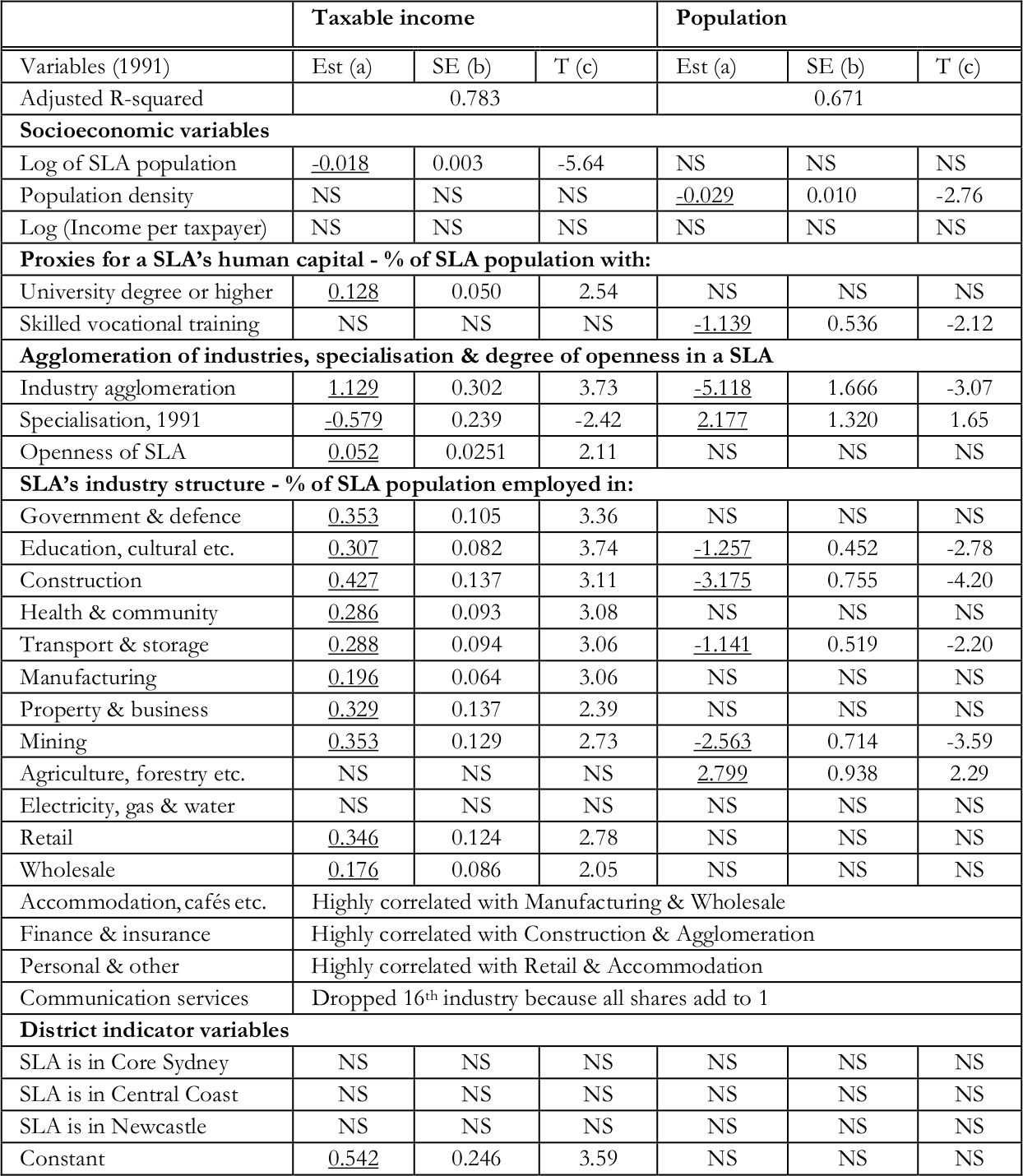
Notes: (a) The regression equations were estimated using STATA linear regression procedure (b) SE stands for standard error of the estimate (c) This column gives T-values computed by dividing the estimate of a coefficient by the standard error of the estimate (NS) Not statistically significant at the 5 % level of significance. Source: Derived by Planning Research Centre, University of Sydney and Bureau of Transport and Regional Economics (BTRE, 2005). 91
Figure 22 is based on a scatter plot of data on taxable income location quotients (with NSW as the reference region) and data on population income location quotients (with NSW as the reference region) for the SLAs in the Sydney GMR.
Figure 22: Scatter plot of strong and weak performing SLAs
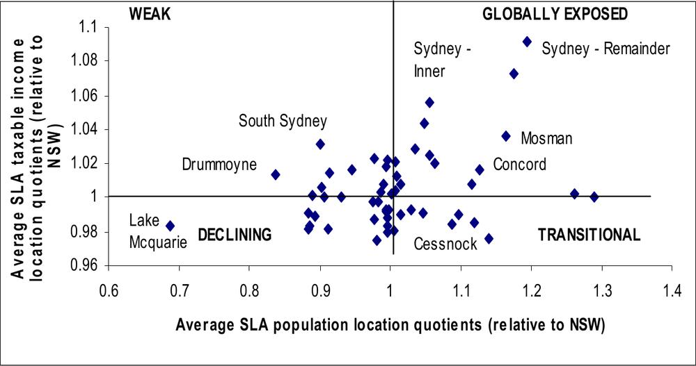
The matrix in Figure 22 provides a summary of current performance and economic options in the Sydney GMR. It shows that strongly-performing SLAs have higher growth in population and taxable income than weakly-performing SLAs. It further groups SLAs into four categories:
- Globally exposed strongly-performing SLAs (based on population and income growth) – these SLAs are listed in the upper right quadrant. They are places which are globally exposed and able to forge a new destiny because they have population and globally oriented specialisation.
- Transitional, modest-performing SLAs (based on population and income growth) – these SLAs are listed in the upper left quadrant. They are places that are getting new people but not yet specialising, usually commuter communities that have not galvanised an economic base. 92
- Static, weak-performing SLAs (based on population and income growth) – this group of SLAs is in the lower right corner. They consist of SLAs with the strongest income bases but that are static in human resources capital. They will need to improve their human capital base to forge a new economic destiny.
- Declining weak-performing SLAs (based on population and income growth) – The lower left quadrant of Figure 21 lists the poorest performers across most dimensions in our study and they are characterised as declining SLAs.
One significant difference between strong-performing and weak-performing regions is in industrial diversity and openness. The average share of manufacturing jobs in total employment in strongly performing SLAs is found to be negative, but the share in knowledge intensive and finance sectors are positively correlated with regional growth. This means SLAs with high values for human capital variables are likely to grow faster. Government employment is an inducer of better economic activity but it does not in itself stimulate a strong economy.
Conclusions
Lang and Blakely (2005) concluded that small suburban areas can be heterogeneous even when they occupy the same regional economic geography. Each small area has endowments from the past (such as industries, natural resources etc.), and each can grow or languish depending on how they capitalise on the past and view the future.
As the techniques we employed show, not all factors are equally important for the economic growth of a small area. Some small areas have human resource assets, while others have manufacturing or retail attributes as building blocks. So, each small area has in essence a recipe for success that differs in some degree with others nearby. Small areas within a greater economic whole such as the Sydney Greater Metropolitan Region can compliment each other and compensate for weaknesses such as human resource capacity, using other assets in fields that represent economic growth (for example, occupations in computer or other technology). 93
Sydney has a strategic advantage in the global economy with its access to sophisticated technology, highly skilled and multilingual labour force. All SLAs in the Sydney GMR, including those with high unemployment, can capitalise on these opportunities through innovative and productive partnerships that build on alliances.
The job market in Sydney GMR is changing rapidly. Manufacturing employment has largely given way to ‘technology & knowledge intensive’ and ‘finance, insurance, property & business services’ jobs that are at the heart of Sydney as a global city – a financial hub linked to all corners of the world. Sydney’s jobs will need to be innovation-related and knowledge-based to support its aging population and compete internationally. Employment is an important factor in determining macroeconomic policy settings.
Although the Sydney GMR as a whole has experienced strong employment growth in the period 1996–2001 (1.6%), there have been some emerging sectoral and spatial imbalances confirmed by this study. The industries of the future in the Sydney GMR need a more educated workforce and the ability to quickly develop and adapt technology. Creativity as a new growth theory is the most important factor of production today. Not surprisingly, it improves labour and capital and extends older resources such as manufacturing, agriculture and engineering as well. What is more, creativity increases the quantity and quality of final goods and services and the latter in turn can enlarge creativity. Finally, creativity tends to increase productivity across all sectors of the local economy.
What a community needs to do is list the strongly and weakly performing sectors in its local economy. Then it can build an economic development strategy, as Blakely and Bradshaw (2003) suggest. Such a strategy would attempt to optimise each area’s attributes and focus on reducing its deficiencies. Thus, a community may need to bolster its industrial diversity even though it has excellent human resources. This brings more science to the process versus the imitation approaches that are frequently used, based on the latest economic development fad.
Figure 18 reinforces the story of small area change within a larger globalising region. Regions, like Sydney, do not globalise evenly across all space. Some areas lag behind because of their historic drags from 94previous industrial structures like mining and steel production. In some cases, previous success in a sector such as Wollongong as a successful steel city will retard the transition to a new economic order. In some respects, having an old economic engine that is highly productive will influence the potential future economic scenarios dramatically as we have shown. So the 1991 economic engine, as our data show, is a predictor of post-1991 success for SLAs in the Sydney GMR. Thus, a community like Newcastle, that underwent a more rapid decline, is able to rebound faster than one that slowly declines. But areas with endowed human capital institutions like hospitals, universities and well positioned land with good housing stocks are better off today and have more options for their economic futures.
Finally, this chapter looked at the regional economy at a fine spatial grain. It used techniques that are simple but powerful for determining economic development. It applied the techniques in a tiered fashion so the vagaries of one analytical template do not give false response or easy answers to complex problems. These techniques can be fashioned to the region changing or shaping its future so that all subareas can be analysed in-depth allowing each of the localities to play a role in the future of the region. The same techniques are useable in monitoring interventions at a micro/suburban area scale overcoming current technical difficulties for assessing differential performance over time to find drivers and alter the performance of lagging areas. In this way, all communities across a metropolitan area can meet the same equitable goals from different economic drivers and economic roots. 95
References
Australian Bureau of Statistics (2002) Sydney: a social atlas based on 2001 Census of Population and Housing. Canberra: ABS.
Barreto, R. A. and Hughes, A. W. (2004) ‘Under performers and over achievers: a quintile regression analysis of growth.’ The Economic Record. 80(248): pp. 17–35.
Blakely, E. J. (1994) Planning local economic development: theory and practice. California: Sage Publications.
Blakely, E. J. (2004) Regional science Cyclops: from a one eye to two eyed view of a changing regional science world. Keynote address to the 2004 ANZRSAI Conference, Wollongong, New South Wales, September 2004.
Blakely, E. J. and Bradshaw, T. K. (2003) Planning local economic development: theory and practice. California: Sage Publications.
Bostic, R. W., Gans, J. S. and Stern, S. (1997) ‘Urban Productivity and factor growth in the late nineteenth century.’ Journal of Urban Economics. 41(1): pp. 38–55.
Bradley, R. and Gans, J. S. (1998) ‘Growth in Australian cities.’ The Economic Record. 74(226): pp. 266–278.
BTRE (2003) Focus on regions no.1: industry structure information. Canberra: Bureau of Transport and Regional Economics.
BTRE (2004) Focus on regions no.2: education, skills and qualifications. Canberra: Bureau of Transport and Regional Economics.
BTRE (2005) Focus on regions no.3: taxable income. Canberra: Bureau of Transport and Regional Economics.
Department of Infrastructure, Planning and Natural Resources (DIPNR) (2005) Sydney metropolitan strategy. Sydney: DIPNR.
Feser, E. J. (2001) ‘Agglomeration, enterprise size and productivity’ in B. Johansson, C. Karlssson and R. Stough (eds.), Theories of endogenous growth. Heidelberg: Springer-Verlag. pp. 231–251.
Goldsmith, W. and Blakely, E. J. (1992) Separate societies: poverty and inequality in US cities. Philadelphia: Temple University Press.
Gujarati, D. N. (1995) Basic econometrics. Singapore: McGraw-Hill.
Hill, E. W. and Wolman, H. L. (1997) ‘City-suburban income disparities and metropolitan area employment: can tightening labour markets reduce the gaps?’ Urban Affairs Review. 32(4): pp. 558–582.
Hoover, E. M. (1937) Location theory and the shoe and leather industries. Cambridge: Harvard University Press. 96
Kasarda, J. D. and Parnell, A. M (eds.) (1993) Third World cities: problems, policies, and prospects. Newbury Park: Sage.
Klosterman, R. E. (1990) Community and analysis planning techniques. Maryland: Rowland and Littlefield Publishers.
Klosterman, R. E., Brail, R. K. and Bossard, E. G. (1993) Spreadsheet models for urban and regional analysis. New Jersey: Centre for Urban Policy Research.
Lang, R. and Blakely, E. J. (2005) ‘Keys to the new metropolis.’ Journal of the American Planning Association. 71(4): pp. 1–11.
Ledebur, L., and Barnes, W. (1992) City distress, metropolitan disparities and economic growth. Washington DC: National Language of Cities.
Marshall, A. (1920) Principles of economics. London: Macmillan.
Massey, D. and Denton, N. (1993) American apartheid: segregation and the making of the American underclass. Cambridge: Harvard University Press.
Mikelbank, B. A. (2005) ‘Local growth suburbs: investigating suburban change in the metropolitan context.’ Opolis: International Journal of Suburban and Metropolitan Studies. 2(1): pp. 1–5.
O’Connor, K. R. (1999) ‘Economic and social change and the futures of Australian metropolitan areas,’ in Benchmarking 99: future cities research conference. Conference Papers, Melbourne City Council, pp. 59–66.
Orfield, M. (1997) Metropolitics. Washington DC: Brookings Institute.
Organization for Economic Co-operation and Development (OECD) (2001a) The well-being of nations: the role of human and social capital. Paris: OECD.
Organization for Economic Co-operation and Development (2001b) Cities and regions in the new learning economy. Paris: OECD.
Organization for Economic Co-operation and Development (2001c) Does human capital matter for growth in OECD countries? Evidence from pooled mean-group estimates. Paris: OECD.
Robertson, E. (2000) Population census evaluation 1996 census data quality: journey to work. Canberra: Australian Bureau of Statistics.
Searle, G. (1996) Sydney as a global city. Discussion Paper: Department of Urban Affairs and Planning and the Department of State and Regional Development.
Stimson, R. J., Stough, R. R. and Roberts, B. H. (2002) Regional economic development: analysis and planning strategy. New York: Springer. 97
Stoll, M. (1999) Race, space, and youth labour market. New York: Garland Publishing.
Toft, G. S. and Stough, R. R. (1986) Transportation employment as a source of regional economic growth: a shift share approach, transportation. Washington DC: Research Board, National Research Council. 98