>meta name="googlebot" content="noindex, nofollow, noarchive" />
6
Management of water resources under uncertainty: what does the future hold?
Abstract
Current predictions indicate that the climate in Australia will become more variable and extreme. This will increase pressure on fragile natural resources and sound water resource management will become increasingly important. Forecasting is therefore essential in both agriculture and natural resource management. Is the current hydrological science up to this task and what tools are available for Australia? Much of the current hydrological knowledge is grounded in the work on perennial and humid systems with virtually no real ‘Australian hydrology’, despite evidence of the unique nature of our semi-arid river systems. While simulation models have become ubiquitous in hydrological science, most are used for so-called backcasting, rather than forecasting. This means simulations are run based on existing daily climate data as future daily predictions are often unavailable and uncertain. Additionally, there is still a significant gap with respect to the data needs of distributed models and the actually available natural resource data. Models with fewer parameters have been advocated, taking full advantage of the information in the available streamflow data. However, the associated simplifications and assumptions also introduce model uncertainties, which should be based on sound systems knowledge. It is unclear how such uncertainties would propagate if the models are used for forecasting rather than backcasting and perturbed under different management scenarios. Research into the temporal variability of model parameters, combined with probabilistic approaches 182to capture the non-linearity and variability of the Australian hydrological system will increase the ability to manage the system into the future.
Introduction
The Australian climate is recognised as one of the most variable in the world (Meinke et al 2003). Given that stream flow is an expression of the rainfall signal, Australian stream flow is also among the most variable in the world (McMahon et al 1992). The latest International Panel of Climate Change assessment foreshadows a significant decrease in water availability in Eastern Australia (IPCC 2007), and the most recent national climate change predictions indicate that the Australian climate will also become more variable (Preston & Jones 2006; Whetton et al 1993). There is also empirical evidence that droughts are becoming more severe, mainly due to changes in temperature (Nicholls 2004). The higher variability in climate implies that increased skill would be needed in forecasting for agricultural production and natural resource planning (Meinke & Stone 2005). Prediction of streamflow, for irrigation and drinking water management, and soil moisture balances, for crop production and irrigation efficiency, will have to be improved. The current drought and its impact on urban and rural water supplies (such as in Goulburn and on the Murray River) indicates that such forward planning is desperately needed. However, the question is on what hydrological scientific information is this forward thinking going to be based? For streamflow and the soil moisture balance, rainfall is the primary forcing variable, but it is the translation that makes prediction of the secondary variables difficult (Kundzewicz & Mata 2007). There is additional difficulty in defining river types, conditions and climatic events. For example, a concept such as drought is not easily defined (Alley 1984; Dracup, Lee & Paulson 1980), and this means that the prediction of drought with increasing variability will be even more difficult.
Much has already been produced in relation to the topic of climate change by colleagues in the field of meteorology and climatology, but it appears that little has been flowing on into the areas of hydrology and agrohydrology. This means that where climatological studies have combined with cropping and hydrological predictions, models have been 183used ‘as is’ (i.e. Chiew & McMahon 2002; Meinke & Stone 2005), and little time has been spent on reassessing the assumptions underlying the models. This chapter will concentrate on an investigation into the nature of hydrological knowledge in Australia and whether this allows us to face future challenges. There is no attempt to review all the literature on this topic. The work mainly focuses on the ability to make hydrological predictions using simulation models under a changing climate.
Australian hydrology
The hydrology of Australia has been identified as being unique in the world (McMahon et al 1992) and is characterised by very low runoff coefficients and high coefficients of variation. Following the classification made by Uys and O’Keeffe (1997), most Australian rivers are episodic, ephemeral or non-seasonal variable, meaning that they can be dry for any length of time during the year. This uniqueness is partly driven by the fact that the Australian environment is mostly arid and semi-arid, which leads to strongly non-linear and highly variable systems. These systems have not been highlighted as much in the hydrological literature as their perennial humid variant. This might be partly due to the difficulty of the topic, partly due to the spatial distribution of hydrologists and partly due to the fact that water resource management of humid rivers is an easier target. While Australian literature has very early recognised that this type of hydrology was different and dominated in many areas of Australia (Pilgrim, Chapman & Doran 1988; Srikanthan & McMahon 1980b; Watkins 1969), this has not led to a significant body of hydrological work, specifically aimed at ‘Australian Hydrology’.
The major thinking in terms of hydrology and the structure of models is based on ideas developed between 1940 and 1960 in the USA and Great Britain (e.g. Beven 2004; Dunne & Black 1970; Freeze and Harlan 1969). The structure of most hydrological models and conceptualised systems can therefore easily be traced back to the work of Horton, Dunne and Freeze and possibly Klemes (Klemes 1978). Much of the traditional hydrology highlights the importance of groundwater driven baseflow (Beven 2001), a component which delivers the persistence and continuity in much of the perennial streamflow. In contrast, semi-arid hydrology is characterised by a rapid response of the streamflow to 184rainfall and only very little persistence (Fig. 6.1). Most Australian rivers are therefore characterised by long periods of no-flow, indicating that the groundwater input is negligible or inconsistent (McMahon & Finlayson 2003). Such a lack of persistence (or baseflow) creates a river system in which streamflow seems almost random and this makes prediction more of a challenge (Pilgrim, Chapman & Doran 1988; Srikanthan and McMahon 1980a; Srikanthan & McMahon 1980b). Most of the hydrological literature discussing Australian catchments builds on the concepts derived from the US and Europe and applies these to the Australian environment. This means that often papers emphasise the contribution of groundwater to the stream flow (e.g. Bari & Smettem 2006; Farmer, Sivapalan & Jothityangkoon 2003; Keith 2004; McMahon & Finlayson 2003; Peck & Hatton 2003; Vaze et al 2004), even though this is unlikely in a semi-arid environment (Pilgrim, Chapman & Doran 1988). Australian books aimed at hydrological practitioners also spend considerable time on the topic of ‘baseflow separation’ and little discussion on semi-arid processes (Grayson et al 1996; Salama 1998; Zhang, Walker & Flemming 2002).
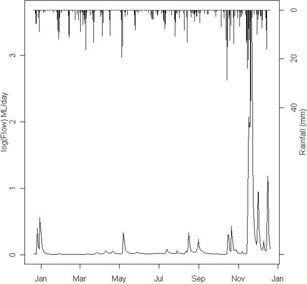
Figure 6.1 Logarithms base 10 of the daily streamflow in megaliters (ML) per day (left axis) and rainfall in mm (right axis) for a semi-arid catchment in northen NSW. Streamflow responds quickly to rainfall, but is a somewhat subdued and delayed reflection of the rainfall. Rainfall is the primary forcing variable, while streamflow is the secondary variable. The flow is plotted on a log scale which exaggerates the low flow behaviour.
185There are two main issues which make semi-arid hydrology particularly challenging:
![]() The highly non-linear response of runoff to rainfall. Depending on the moisture status of the catchment, a similar amount of rainfall can generate totally different levels of runoff (Pilgrim, Walker & Doran 1988). This leads to difficulties in simulating rainfall runoff response.
The highly non-linear response of runoff to rainfall. Depending on the moisture status of the catchment, a similar amount of rainfall can generate totally different levels of runoff (Pilgrim, Walker & Doran 1988). This leads to difficulties in simulating rainfall runoff response.
![]() The nature and variability of the transmission losses (Dunkerley & Brown 1999; Knighton & Nanson 1994; Lange 2005). This leads to difficulty in simulating the routing of streams through a catchment.
The nature and variability of the transmission losses (Dunkerley & Brown 1999; Knighton & Nanson 1994; Lange 2005). This leads to difficulty in simulating the routing of streams through a catchment.
On the other hand, there is a body of work, mainly related to the ecology and geomorphology of rivers in semi-arid regions of Australia, that recognises the variability and unpredictability of flow (Costelloe et al 2003; Dunkerley & Brown 1999; Knighton & Nanson 1994, 2001; Thoms & Sheldon 2000; Young, Brandis & Kingsford 2006). Other authors have highlighted the unique connection in time between streamflow and the El-Niño Southern Oscillation signal (ENSO), particularly in south eastern Australia (Chiew et al 1998; Piechota et al 1998). The ENSO is related to the southern oscillation index (SOI) and the annual fluctuation in temperature of the ocean water of the coast of South America. High ocean temperatures near South America are related to negative SOI indices and are generally related to dry years or drought conditions in Australia and vice versa (see http://www.bom.gov.au/climate/enso/). 186As a result, the amount of streamflow appears to follow the SOI signal up and down with about a 3-month lag (Chiew et al 1998; Piechota et al 1998). However, all stations used for the above-mentioned research were relatively close to the ocean in the zone defined as humid (Watkins 1969), with no stations in the more arid interior. If the aridity and with it the variability of the rainfall increases, drought signatures persist longer in soil moisture (Entekhabi, Rodriguez-Iturbe & Bras 1992). As riverflow will only occur at high soil moisture levels (i.e. there has to be ‘too much’ water) this would decrease the connection to the ENSO signal, meaning the river flows would either not follow this signal as strongly, or not at all.
Overall, it seems that the uniqueness of Australian hydrology is recognised, but that researchers have struggled to come to terms with these difficulties in terms of conceptual models and predictions. Development of future management will need to be based on a good understanding of the hydrological system. Further research into semiarid hydrological systems and their behaviour under a range of conditions appears to be an important need for Australia.
Simulation models and forecasting
To be able to develop management decisions, simulation models are key as they allow predictions into the future. There has been much debate in hydrological science on how well models actually predict the behaviour of a system and the uncertainty that is related to the predictions of models (Beven 2002; Kirchner 2006; Silberstein 2006). In general, the conclusion is that while models are not perfect, they are the best possible means of studying systems. Basically, hydrological models are based on the conceptual image a scientist has of the catchment and this is translated into a set of mathematical equations and computer codes. The model needs three types of data: the first are boundary conditions and initial conditions, the second are parameters, which are generally considered to be time-invariant and define the internal processes in the system; the third are variables, which force the behaviour of the model (such as rainfall and potential evaporation). The model output is then compared against observed data and the parameters in the model are 187adjusted (this is the process of model calibration) to get the best possible match between observed and predicted data.
Hydrological models aim to forecast the variable of interest (in most cases stream flow or groundwater) for management purposes. This means they attempt to look into the future to see how different actions will influence the variable. Interestingly, most scenarios and hydrological models only backcast (or hindcast) that is; the forcing variables (i.e. rainfall) tend to be based on existing measurements, with the argument that these data are more reliable (Stauffacher et al 2003; Tuteja et al 2003; Vertessy et al 1993). This means that the models tend to simulate a different realisation of the current or historic time, rather than look into the future. This approach appears to be the most common in analyses of management impact on stream flow.
A different approach is taken by most research interested in climate change. In those cases the output of global circulation models (GCM) is downscaled to the scale of interest and the different climate scenarios are pushed through hydrological models (Jones et al 2006), often calibrated earlier using historical data (e.g. Chiew et al 1995). While this seems a better approach, as it recognises the fact that we cannot use the current climate to predict future impacts, it still has some problems. One important issue is that the downscaled GCM data for the future is not very accurate and daily estimates are difficult to obtain (Chiew 2006).
Time invariance of parameters
Another issue relates to the underlying assumptions on which hydrological models are based. Different rainfall runoff model structures have different responses to changes in rainfall (Boorman & Sefton 1997; Jones et al 2006). Depending on how the conceptual rainfall-runoff model is structured and how this is translated into code, the runoff response to rainfall will differ. Apart from the more complex distributed groundwater and surface water models, most hydrological models consider parameters to be time invariant. This means the ‘calibrated’ parameter values of the model will be based on historic data, and assumed to undergo no change into the future. However, the parameters in hydrological models are generally coupled to some conceptual representation of the soil or vegetation system or the routing parameters 188in the catchment. Studies to investigate the sensitivity and uncertainty of parameters help explain some of the model outcomes (Boorman and Sefton 1997; Jones et al 2006), but this does not recognise a further problem (Boorman & Sefton 1997; Chiew et al 1995), which is caused by the coupling and feedbacks between climate, vegetation, soil moisture and streamflow.
Because soil moisture and stream flow are dependent secondary variables (Fig 6.1), the behaviour is dependent on changes in vegetation and climate. The work by Eagleson and Entekhabi (Eagleson 1978; Eagleson & Segarra 1985; Entekhabi, Rodriguez-Iturbe & Bras 1992) has highlighted that such feedback loops can be strong, and this would undoubtedly influence results (Chiew et al 1995; Farmer, Sivapalan & Jothityangkoon 2003). What this means is that it is highly unlikely that parameters are time invariant, and this is often demonstrated during calibration and validation (e.g. Kirchner 2006). During calibration, the model parameters are in fact adjusted to the ‘mean’ value of the time series of the ‘true’ parameters, or in other words, the calibrated parameters can be seen as the expected value of the parameter distribution. While this is recognised in model calibration and is the basis of the thinking behind equifinality (Beven 2002), the implications of this for forecasting under climate change scenarios seem to be less recognised. For forecasting under changed climate the variability of the parameters in time needs to be predicted.
Of course, it is difficult to predict how model parameters will change into the future. I am not advocating that an ‘evolutionary model’ should be created that will adapt to changes. Such a model would be too complex and the number of relationships and parameters within the model would not allow a calibration or validation (Kirchner 2006). However, as a minimum requirement, long-term forecasts should analyse whether the distribution of parameters during the calibration period will be the same as the distribution during the forecast period (e.g. Evans & Schreider 2002). Given the complexity in the catchment scale processes and the number of feedback loops, this will probably not be true.
189Research into the variability of model parameters in time, their sensitivity to climatic and weather indices and their biophysical explanation has so far not been extensively attempted. The work by Evans and Schreider (2002) and Wilby (2005) are possibly the only papers making an attempt. The analysis by Evans and Schreider (2002) (which found no significant change in parameters) was limited to only one catchment on the coastal fringe in Western Australia, while their climate change modelling included six catchments. In contrast, the work by Wilby (2005) is more thorough, but the work was done on the Thames River in England.
What is needed are relationships that will predict changes in the model parameters with time, climate or weather, such as southern oscillation index (SOI), rainfall, temperature and carbon dioxide (CO2) levels. This would thus extend the more common sensitivity analysis to actual predictive relationships. It seems somewhat contradictory: to use a model to predict the parameters of a model. However, empirical relationships, kriging, pedotransfer functions (McBratney et al 2002) and meta modelling (Haberlandt, Krysanova & Bardossy 2002) are already established approaches to derive or integrate parameters for simulation modelling. Though these methods mostly predict spatial model parameters, it justifies the study of a similar approach in time-dependent parameters. This explicitly recognises the dynamic nature of many of the soil and vegetation parameters and their influence on the hydrology of a catchment.
Distributed models and data
In semi-arid and arid catchments, simulation modelling is made difficult by the earlier mentioned non-linearities. For example, while the longterm non-linearity in rainfall-runoff can sometimes be accounted for by equating the mass balances (Jakeman & Hornberger 1993), this would not account for the possible dynamic nature of such a non-linearity. This can only be accounted for by explicitly modelling the water balance and drying in the catchment, such as by using and predicting the catchment moisture balance (Croke & Jakeman 2004; Evans & Jakeman 1998).
One approach to improve the modelling outcomes in arid and semi-arid catchments would be to increase the complexity of the model and to 190explicitly include the different processes. This is the direction in which many hydrological models have gone, following the concepts developed by Freeze and Harlan (1969). There are, however, difficulties with this: such an increase in complexity has to be matched with an equivalent increase in data available for parameterisation, calibration and validation. While some aspects can be included with few additional parameters (Croke & Jakeman 2004), more complex interactions and processes would require more data.
The difficulty is that Australia and semi-arid areas in general are relatively data poor. Again, this is partly due to the extensive nature of the human activities in such areas, which means they are less densely populated and economically less important. In addition, the large land mass of Australia has also limited data collection, purely due to the related costs. Only in recent years, with the development and availability of satellite and remote sensing data, do we see an increase in data availability. However, the relationships between remotely sensed data and hydrologically important variables are still tenuous (Schmugge et al 2002; Western et al 1999). Increased calibration and validation data in the form of streamflow is also difficult as most gauge records are not long enough to cover all variability. The fact that zero flows cannot be used as calibration data and that these occur frequently does not help the situation (Pilgrim, Chapman & Doran 1988).
Complexity or simplicity
There are generally two reasons for increasing the complexity in a model. The first is to increase the accuracy of the predictions; the second is to gain more insight into the processes. In the context of climate change and future predictions, the first seems more important. However, a range of authors have argued, and demonstrated, that increased complexity does not equate to increased accuracy of prediction (e.g. Beven 2001; Grayson, Moore & McMahon 1992; Jakeman & Hornberger 1993; Silberstein 2006; Sivapalan 2003). This has led to several researchers arguing for a so-called ‘top-down’ approach, which starts with a basic model of the catchment and increases in complexity when necessary (Farmer, Sivapalan & Jothityangkoon 2003; Sivapalan et al 2003; Young 2003), purely based on the information in the flow data set. This is attractive in terms of decreasing the need for parameters and 191delivering statistically sound predictions and their uncertainties. In addition, each increase in complexity should deliver additional information about the behaviour of the catchment (Sivapalan 2003).
While we can use statistics, such as the Akaike Information Criterion to maximise the parsimony in models, this comes at a cost not quantified in the statistic. This assumes that the understanding of the hydrological processes is sufficient to develop conceptual models. The simpler models might include conceptual simplification, which might or might not represent the true complexity and behaviour of the system. If this is not the case then calibration is no more than extensive curve fitting, which lowers the confidence in the outcomes. While the model might be more parsimonious in the calibration period and fit the data better, this does not always translate to a validation period (Refsgaard & Henriksen 2004). This can often be seen in the difficulty in validating models; while a model can often be well calibrated, validation is not easily achieved (Refsgaard & Henriksen 2004). Understandably, if the model is subsequently perturbed with quite different climate data from a climate change scenario, there is no guarantee that the historical parameter data are valid for the future periods (e.g. Boorman & Sefton 1997; Wilby 2005). Many of the papers using the “top-down” approach are limited to calibration (e.g. Farmer, Sivapalan & Jothityangkoon 2003; Jothityangkoon, Sivapalan & Farmer 2001; Son & Sivapalan 2007), although the last paper uses a range of different data (such as water quality and quantity). Only solid conceptual understanding will allow simplification of complex models, but conversely the understanding can only be achieved using more complex and data-rich models, and this needs to be regularly checked and updated.
Example 1: Soil moisture balances
Part of the inspiration for this chapter was given by a debate about the occurrence of drought and the definition of drought in northern NSW. The debate focussed on the question whether it was the rainfall deficiency or the rainfall variability and timing that defined the occurrence of drought. From an agricultural or natural resource planning perspective the latter is more important than the former. This means that the definition of drought is somewhat nebulous and the future 192prediction of drought even more so. The literature is quite similarly undecided about the definition of drought (Alley 1984; Byun & Wilhite 1999; Dracup, Lee & Paulson 1980; Hisdal & Tallaksen 2000; Whetton et al 1993) and different calculations procedures have been suggested to calculate the occurrence of drought. These procedures differ depending on the perspective, for example, we can define a hydrological, an agricultural and a socioeconomic drought (Dracup, Lee & Paulson 1980). An ‘exceptional circumstances’, declaration by the federal and state governments in Australia can be seen as a declaration of socioeconomic drought (Donnelly, Freer & Moore 1998).
For future agricultural management, it seems most important to focus on the probability (likelihood) of a soil moisture deficiency at critical times. Soil moisture deficiency has often been suggested as a more objective agricultural drought criterion than rainfall deficiency, and calculation examples have been developed (Byun & Wilhite 1999; Hisdal & Tallaksen 2000). The well-known Palmer Drought Index is also based on some sort of soil water balance (Alley 1984). The problem in this case is the issue of regionalisation. While it is not difficult to calculate the changes in soil moisture over time at a point in the landscape, it becomes difficult to extend these results to a larger region or across regions (as the Palmer drought index attempts) as spatial variability of soils and vegetation would affect the results. By using a probabilistic system, such differences can, of course, be accounted for through the related uncertainty.
The calculation of statistical moisture distributions is not new; in fact there are a series of papers dealing with this concept beginning with Eagleson (1978). The concept has later been extended (Entekhabi, Rodriguez-Iturbe & Bras 1992; Laio et al 2001; Milly 2001; Rodriguez-Iturbe 2000) to allow calculation of crossing probabilities and plant water stress. The advantage of these approaches is that they are based on an analytical model and this allows direct calculations of distribution of values (the probability density function) and the mean and variance of the variable in question. These properties give a summary of the values, the probability density function gives a graphical overview of the distribution of values, which can also be described by such statistical parameters as the mean, variance and skewness. It also allows the 193calculation of the likelihood (probability) that something might or might not occur. In this section, an example of the calculation of the probability of a certain soil moisture status will be given for two different soils in two locations in NSW.
Methods
Two rainfall datasets from 1901–1998 were extracted from Rainman V4.3 (Queensland DPI, Brisbane, QLD) for a site in the north west of New South Wales (NSW) (Warialda Creek station 418016) and a site in central west NSW (Lachlan River station 412063). Monthly evaporation data were obtained from the Bureau of Meteorology website (http://www.bom.gov.au). The two sites have some differences in their distributions of rainfall and evaporation (Table 6.1), with the Lachlan site being slightly higher in rainfall and daily evaporation, but with a narrower and less skewed distribution.
Table 6.1 Statistics of rainfall and evaporation for Warialda and Lachlan stations used in example 1
| Warialda | Lachlan | |
|---|---|---|
| Mean daily rainfall depth | 1.85 | 1.95 |
| Mean dry spell length | 0.27 | 0.38 |
| Variance daily rainfall depth | 33.2 | 26.7 |
| Skew daily rainfall depth | 6.58 | 5.61 |
| Mean daily Evaporation | 2.73 | 3.12 |
| Variance daily Evaporation | 2.14 | 1.97 |
A soil moisture balance model, such as suggested by Milly (2001), was used to calculate the daily ‘relative’ soil saturation (scale of 0 to 1) for both locations. The relative soil saturation (s) is defined as:

194Where, θ is the soil water content, θw is the water content at the wilting point and θs is the saturated water content. This was used to derive the numerical probability density function of the relative soil saturation for both locations on two representative soil types (medium light clay and clay) and two different profile depths (Zr) (Table 6.2). This means, daily values of soil moisture were calculated for 96 climate years and these were summarised in the probability density function.
Table 6.2 Parameters for the Milly (2001) soil moisture balance model for the medium light clay (MLC) and clay used.
| Medium light clay (MLC) | Clay | |
|---|---|---|
| Zr (mm) | 500, 1000 | 500, 1000 |
| N | 0.43 | 0.37 |
| s1 | 0.86 | 0.72 |
Note: The parameter Zr represents the root or profile depth, n is the porosity and s1 is the soil saturation at which runoff occurs.
The rainfall datasets were also used to derive the mean dry-spell length and the mean rainfall depth assuming the rainfall events follow a Poisson distribution (Rodriguez-Iturbe, Gupta & Waymire 1984) (Table 6.1). This is then used to derive the theoretical probability density function of the relative soil saturation (Milly 2001). In this case, the daily values were not actually calculated as the values for the probability density function can be calculated directly.
Results
All the probability densities functions (pdfs) for the relative soil saturation indicated a strong peak (maximum) at the dry end (Fig. 6.2). This means that the soil is ‘most likely’ very dry. Note that 0 does not mean that the soil is bone dry, rather in this model it indicates that the soil is at the dry end of the soil saturation spectrum (wilting point) and water available for plants will be very limited. The strong peak at the dry 195end would be expected, given that both these areas can be classified as semi-arid.
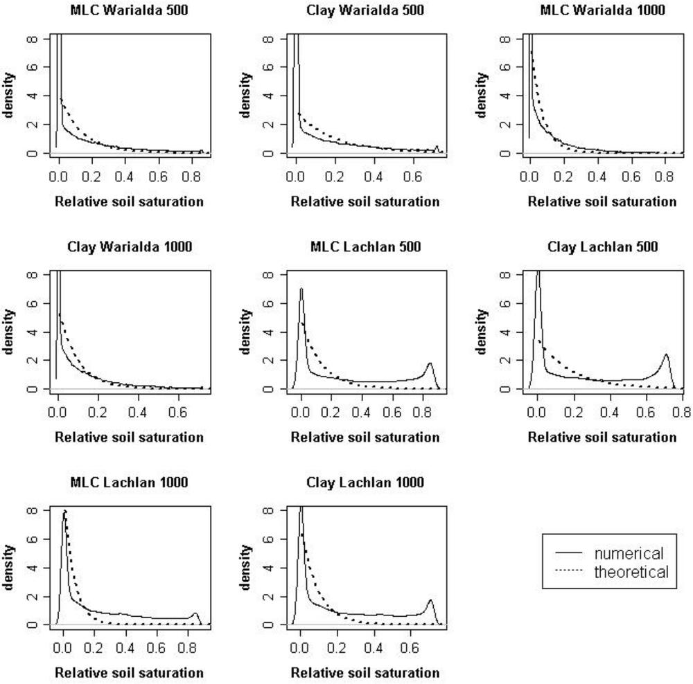
Figure 6.2 Numerical and theoretical probability density functions (pdfs) for the two locations, different soil types and different root depths. The y-axis gives the relative frequency of occurrence with large values indicating more probable values. A large peak (maximum) can be observed at the dry end (around zero), particularly for Warialda, but particularly the graphs for the Lachlan location indicate a bimodal structure, with a second (smaller) peak near saturation, indicating two preferred soil moisture states (Western, Blöschl & Grayson 2001). 196
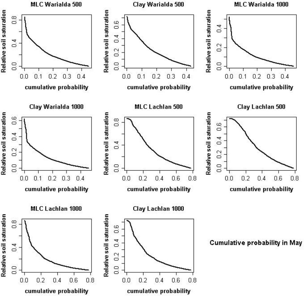
Figure 6.3 Cumulative distributions of relative soil saturation in May for the two locations and different soils and root depths. The results indicate that there is generally a low probability that the relative soil saturation would be above 0.5 (or half full moisture profile) at both locations.
The theoretical pdfs are even more skewed than the numerical pdfs, meaning that they indicate even stronger the fact that the soils are ‘most likely’ dry. The means and variances of the numerical distributions are much higher than the theoretical distributions, indicating that the theoretical distributions probably underestimate the probabilities (likelihood) of the soil being wet and overestimate the probability associated with the dry end. However, overall the shape of the 197theoretical pdfs is similar to the numerical pdfs, particular for the Warialda location.
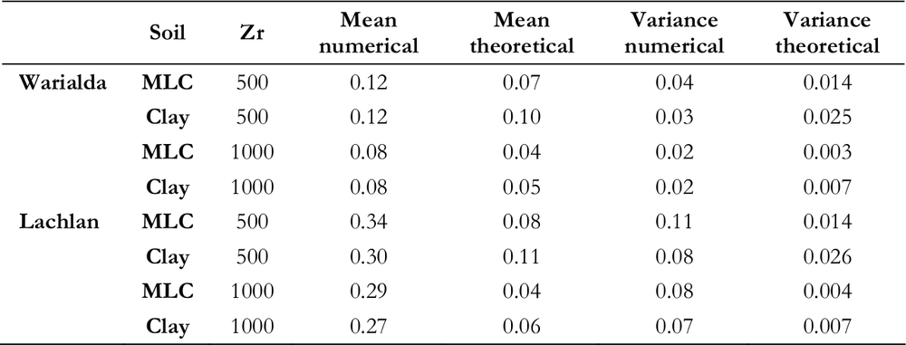
Interestingly, the Lachlan distributions are bimodal with a second (smaller) peak occurring at the wet end (Fig. 6.2). This indicates that the soil will also be at the wet end for significant intervals, but does not spend much time at the intermediate levels (Western, Blöschl & Grayson 2001). Similar responses for a semi-arid climate have also been indicated by Entekhabi, Rodriguez-Iturbe & Bras (1992) and this has been related to the fact that a significant shock is needed to move from a drought (low moisture) to a wetter regime and vice versa. The results indicate that the Warialda location is less likely to have significant soil moisture during the year and is more likely to have a dry profile. Overall the results indicate that, based on the data of the last century, the soil in Warialda has been more often dry than wet, while the Lachlan soils had a bit higher likelihood of having some soil moisture and this is also reflected in the means of the distributions (Table 6.3). This has, of course, serious implications for agricultural management. The theoretical means agree better with the numerical results in the drier location (Warialda, Table 3), again indicating the underestimation of the soil saturation. The fact that the numerical pdfs in the drier location agree reasonably with the theoretical pdfs means that the theoretical pdfs could also be used to calculate broad statistics for the average relative soil saturation status.
Table 6.3 Statistics for the numerical and theoretical pdfs for the different soil types and root depths at the Warialda and Lachlan stations.
Note: MLC is medium light clay, Zr is the root depth.
198The same results can also be analysed using a cumulative distribution. This allows the estimation of the probability of having a certain soil saturation level (for example needed for planting crops or to estimate runoff potential of predicted rainfall) for the different soils. In relation to planting crops, the most crucial time for wheat production is the soil moisture status in May, when most growers would like a full- or half-full soil moisture profile for planting. Using the data from the soil moisture balance and plotting the cumulative probabilities of relative soil saturation for the month of May, it is clear that the prospects of having sufficient moisture for wheat planting (i.e. 50% full or higher, or above 0.5 on the y-axis) are in fact quite slim (Fig. 6.4). Probabilities are generally small (below 20%), indicating that, in essence, sufficient soil moisture for planting can only be expected one in five years. Given the limited number of soils and the simple soil moisture model applied, this is of course a somewhat uncertain estimate.
The analysis however indicates two major points. The bimodal behaviour indicates that the soil moisture status basically revolves around two states, one wet and one dry (i.e. Western, Blöschl & Grayson 2001). Significant weather changes (such as a ‘La Niña’ or ‘El Niño’ event) are needed to move from one state to the other. This also means that after a prolonged dry period, there remains a significant probability of returning to the dry soil moisture status even after some rain. Secondly, the use of the cumulative probability distribution allows an assessment of the ‘average’ risk for agricultural production in the area. It indicates the probability of a certain moisture profile in the future, purely based on the historical climate data and the soil properties.
Under climate change, the distributions would of course shift, but as the model does not involve any calibration, but is based on the ‘average’ soil characteristics in the area, there would be little change in the soil parameters. The difficulty of generating representative daily rainfall data from climate change scenarios to drive the model remains (Chiew 2006). However, while in this case the rainfall amount, as well as the daily distribution is important, a stochastic realisation of the rainfall data would be sufficient. 199
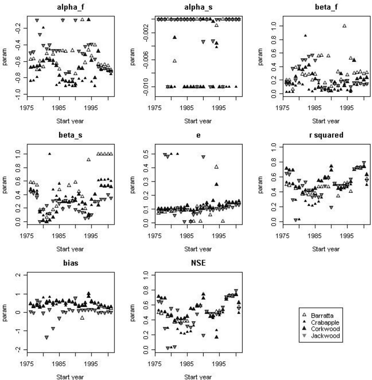
Figure 6.4 Variation in calibrated parameters for five-year moving windows for four of the catchments in the Karuah Hydrology Research catchments from 1976 to 2005. Parameters are plotted against the start year of the moving window. Some of the parameters are clearly highly variable in time, while others are relatively stable.
Example 2: Temporal variability of model parameters
NSW State Forests has a long-term monitoring program on a series of research catchments on the mid-north coast of NSW, near Chichester on the headwaters of the Telegherry River. These catchments, the 200Karuah Hydrology Research, were originally set up to study the effect of logging on catchment water yields (Cornish 1993). Some of the catchments were logged in 1983, while others have never been logged (Cornish 1993). Two earlier papers describe the changes in the catchment water yield and the changes in evapotranspiration as a result of the logging treatments (Cornish 1993; Cornish & Vertessy 2001). This example will not research that aspect, but the good quality streamflow data for the catchments, which is available from 1976 to 2005, creates an opportunity to study the temporal variability of parameters in a rainfall-runoff model.
Methods
The data were subdivided into five-year moving windows and a rainfall runoff model, the CMD version of IHACRES (Croke & Jakeman 2004; Evans & Jakeman 1998), was used to predict the streamflow over each period for the first four catchments. Of these, three have been logged, while the Crabapple catchment has never been logged (Cornish 1993). Maximum temperature was used as a proxy for potential evaporation (Croke & Jakeman 2004; Evans & Schreider 2002) and rainfall was sourced from the nearby Chichester dam weather station. The CMD version of the IHACRES model has a total of eight parameters that describe the streamflow response of the catchment. Three of the parameters can be readily fixed (Croke and Jakeman 2004) and these are: f, which is the ratio between the flow and the stress thresholds, d1 (mm), which is the flow threshold and n, the balance between the two linear segments of the drainage equation. Of the other five parameters, four describe the balance between quick flow (f) (generally direct runoff) and slow flow (s) (often groundwater input): alpha f and alpha s, the decay parameters (unitless) for the quick and slow flow and beta f and beta s, parameters (unitless) which determine the fractions of quick and slow flow in the final output (for a full description see Croke & Jakeman 2004). The final parameter is e (unitless or mm/°C), which determines the transformation of the daily evaporation (or daily maximum temperature) to evapotranspiration.
Following the suggestions by Croke and Jakeman (2004), the last five mentioned parameters were calibrated (Table 6.4) using a five-year moving window over the data (i.e. 1976–1981, 1977–1982, 1978–1983, 201etc.). This means 26 five-year datasets were used, which all partly overlapped with their neighbours. Parameter uncertainty was not analysed here, but this could add additional complexity (Wilby 2005). The parameters were calibrated by matching the observed flow data to the predicted flow data and by maximising the Nash-Sutcliffe Efficiency (NSE). The NSE is a standard measure for goodness of fit in hydrology and is defined as 1 minus the ratio of the variance of the observed minus predicted data divided by the variance of the observed data (Beven 2001):

Values of NSE close to 1 indicate a good fit, while 0 or negative values indicate that the model is no better than fitting the average value.
Table 6.4 Overview of calibration parameters for the CMD IHACRES model.
| Parameter | Initial value | Upper bound | Lower bound |
|---|---|---|---|
| alpha f (-) | -0.7 | -0.1 | -1 |
| alpha s (-) | -0.01 | -1E-10 | -0.01 |
| beta f (-) | 0.5 | 1 | 0.001 |
| beta s (-) | 0.5 | 1 | 0.001 |
| e (mm °C-1) | 0.15 | 1 | 0.01 |
| f | 0.93 | Fixed | |
| d1 (mm) | 200 | Fixed | |
| n | 0.1 | Fixed |
Note: The f (ratio of the flow and stress thresholds, d1 (the flow threshold) and n (the balance between the two linear segments of the drainage equation) parameters were fixed (Croke & Jakeman 2004).
Results
Some of the calibrations of the model were not very good with NSE values ranging from negative (indicating no fit) to 0.79 (indicating a good fit) (Fig 6.4). This ‘goodness of fit’ is also expressed by the r-squared (which indicates the correlation between observed and predicted) and 202the bias (in mm, which indicates how much the model over or under predicts) (Fig. 6.4). However most of the fitted parameters indicate temporal variability (Fig. 6.4). Given that some of the calibration results were quite low, it means that the results of this study should be interpreted with some caution.
The variation in some of the parameters (such as the quick flow parameters, alpha f and beta f) is quite substantial (Fig. 6.4). In practice this would translate in varying amounts of quick flow (or streamflow which quickly responds to rainfall) being predicted over time. This variation is no different for the catchments which were logged and the catchment which was not logged (Crabapple). The lowest variance is in the Barrata catchment, which also had the lowest change in water yield following logging (Cornish 1993). In contrast, the unlogged Crabapple catchment has the highest variation. This already indicates that the assumption of temporal parameter stability is clearly untenable, even without the land use effects included in these data. Similar variation in parameters in time in rainfall-runoff modelling were also found in a calibration and validation example for the Thames River (Wilby 2005) and is often encountered when attempting to validate models, indicating that this result is not isolated.
Some interesting points can be observed from the data. The variance is largest in the quick flow parameters alpha f and beta f, which describe how fast and what fraction of the runoff directly responds to rainfall. The variation in the alpha s parameter is the lowest, but this might be partly caused by the fact that the parameter was only allowed to vary over a small range during the calibration (Table 6.4).
Another interesting fact is the low calibration results obtained for all catchments in the 1980s (around 1985). This was the period that most of the catchments were logged (Cornish 1993), but it also includes the drought in that period (1980) and the period right after, which included high flows (1983–1985) (Cornish 1993). During this period, the model has difficulty in predicting the observed data in all catchments, including the catchment that was not logged. The low calibration results (and related change in the alpha f and beta s parameters) could be caused by a wide range of landscape and climate properties, and this in itself would 203be an indication of parameter variability in time (Fig. 6.4). It could also be a case of measurement uncertainty, with the results reflecting possible inaccuracies in the data in that period, as the logging activities might have disturbed some of the measurements.
Interestingly, a slight positive trend with time can be observed in the e parameter (Fig. 6.4). This parameter is related to evapotranspiration from the catchment (Croke and Jakeman 2004), with increasing e indicating an increase in the predicted evapotranspiration. The slow increase after logging in 1983 is not surprising, as the regrowth would increase evapotranspiration (Cornish 1993). However the e parameter for the unlogged Crabapple catchment also increases and the increase is over the whole period of measurement (both before and after logging), which would not be expected. The results are therefore possibly some indication of climate effects at a much longer time scale. This could indicate that temporal parameter variability itself can be a tool for investigating long-term climatic trends or cycles.
Summary and discussion
Climate change will create some significant challenges for Australia in terms of water, natural resources and agricultural management. These challenges will have to be anticipated to be managed, and this anticipation can best be based on solid simulation modelling results as these offer the best possibility to predict the future. However there are some significant gaps in our current modelling capabilities. Many of those have been highlighted by other authors and have only been summarised in this chapter (Beven 2002; Chiew 2006; Kirchner 2006; Silberstein 2006). As a result, models are often calibrated, but not validated and most models are used in a back- or hind-casting manner which does not enable reliable predictions into the future for two reasons: the climate data are not representative of the future; and the parameters in the model cannot be assumed to be time invariant into the future (see example 2).
The problem is further exacerbated in Australia due to the low data availability in large areas and the non-linearities in the semi-arid system. Semi-arid hydrology and ‘Australian hydrology’ have, in addition, not 204been studied in a coordinated and focussed manner, with much of the current hydrological knowledge in Australia still strongly grounded in humid US and European theory. This appears to neglect the unique nature of the Australian systems.
For management purposes and due to data paucity, simplified models (Stauffacher et al 2003) have been advocated in Australia and this should also enable better calibration and lower parameter uncertainty (Sivapalan 2003; Young 2003). However, simplification of models can only occur if such simplification is valid and robust, based on the best possible conceptual models, and will account for most variability in the systems. The best example of a successful simplification is probably the so-called ‘Zhang curves’, which are relationships between rainfall and evapotranspiration for different vegetation types (Zhang, Dawes & Walker 2001). These curves are based on a thorough understanding of the underlying conceptual model, and give a quick estimate of the elements of the hydrological balance, such as deep drainage and runoff. Danger occurs when conceptual models are based on theory developed elsewhere, which is not checked against local observations. Too much simplification will mostly just deliver the long term expected value. Since ‘variability’ is the key word in Australian hydrology this may be problematic.
Overall, this seems to suggest that there are some significant difficulties in terms of using models for making predictions of future trends in water, natural resources and agriculture for Australia. The tools are still lacking, but there are also some deeper conceptual difficulties related to semi-arid hydrology, which partly relate to social training and distribution of hydrologists. Development of a uniquely Australian hydrological science which focuses specifically on the particular issues of semi-arid hydrology and is supported by a strong data collection program (Silberstein 2006) appears to be a prime need for the future.
Risk and probability are important concepts for future management. Being able to assess the risk or probability of success of certain management activities will assist in making policy decisions. Particularly in the case of highly variable properties, such as soil moisture or streamflow, probabilistic approaches can give a better indication of the 205most likely magnitudes of a property. In the case of soil moisture (example 1) it can be used to assess the probability of having sufficient moisture for planting or for completing a crop. The cumulative probability curve in the example clearly indicates that ‘dry’ is the norm, rather than the exception.
Future predictions with models hinge on the ability of the model to capture the main dynamics and feedbacks of the catchment under changing climate. One of the problems with forward prediction, real forecasting, is that any uncertainty in the conceptual model will be propagated in the forecast, even if the model is calibrated on historic data. This means that forecasting validation is essential, and should in particular cover a data set with a different variability to the calibration set. However, this is seldom done in practice, either due to unavailability of the validation data, or because it is just too difficult. What is demonstrated in example 2 is that assuming that parameters are variable in time might assist in developing better calibration and validation of models. Given the semi-arid character of the Australian hydrology and its strong non-linear response to rainfall, temporal variability of model parameters would be logical and the runoff response would be highly likely to change under different climatic conditions due to the strong vegetation response in semi-arid systems and the strong feedback between vegetation and hydrology. However, if there is a trend in the data with time, land use or with climate indices, then this might be translated into temporal variability of the parameters. This can be used to derive relationships, which can be applied in climate change scenarios. What isn’t researched here is the interaction between parameter uncertainty and temporal parameter variability. Note that the former has been researched extensively, but the second has not attracted attention. The question is whether using time variant parameters will reduce parameter uncertainty. This will be the topic of further research in this area.
Conclusions
Climate change is creating some significant challenges in hydrology and these challenges are made even more difficult due to the unique non-linearity and high variability of the processes in Australian semi-arid 206systems. Development of a strong branch of Australian hydrology to focus on the specifics of such systems is needed. Two areas of further research in this context have been identified. Firstly, continuing to develop probabilistic approaches which can be translated easily into risk for management purposes and, secondly, investigating parameter variability in time and uncertainty in rainfall-runoff and other hydrological models to better manage the dynamics of semi-arid systems. Both of these are needed to develop credible scenarios for natural resource management under climate uncertainty.
Acknowledgements
The author would like to acknowledge Dr Ashley Webb from NSW State Forests for kindly sharing the data from the Karuah Hydrology Research, Floris van Ogtrop for fruitful discussions on these topics and Zara Farrell and Leah McKinnon at the BRG CMA for asking critical questions about drought and soil moisture balances. 207
References
Alley W M, 1984. The Palmer drought severity index: limitations and assumptions. Journal of Climate and Applied Meteorology, vol. 23, pp. 1100–1109.
Bari M A, Smettem KJ 2006. ‘A conceptual model of daily water balance following partial clearing from forest to pasture’, Hydrology and Earth Systems Sciences, vol. 10, pp. 321–337.
Beven K J, 2001. ‘Rainfall-runoff modelling: the primer’, John Wiley & Sons, Chichester.
Beven K J, 2002. ‘Towards and alternative blueprint for a physically based digitally simulated hydrologic response modelling system’, Hydrological Processes, vol. 16, pp. 189–206.
Beven K J, 2004. ‘Robert E. Horton’s perceptual model of infiltration processes’, Hydrological Processes, vol. 18, pp. 3447–3460.
Boorman D B & Sefton C E M, 1997. ‘Recognising the uncertainty in the quantification of the effects of climate change on hydrological response’, Climatic change, vol. 35, pp. 415–434.
Byun H R & Wilhite D A, 1999. ‘Objective Quantification of Drought Severity and Duration’, Journal of Climate, vol. 12, pp. 2747–2756.
Chiew F H S, 2006. ‘An overview of methods for estimating climate change impact on runoff’, in ‘3rd Hydrology and Water Resources Symposium’, Launceston, TAS.
Chiew F H S & McMahon T A, 2002. ‘Modelling the impact of climate change on Australian streamflow’, Hydrological Processes, vol. 16, pp. 1235–1245.
Chiew F H S, Piechota T C, Dracup J A & McMahon T A, 1998. ‘El Nino/Southern Oscillation and Australian rainfall, streamflow and drought: links and potential for forecasting’, Journal of Hydrology, vol. 204, pp. 138–149.
Chiew F H S, Whetton P H, McMahon T A & Pittock A B, 1995. ‘Simulation of the impacts of climate change on runoff and soil moisture in Australian catchments’, Journal of Hydrology vol. 167, pp. 121–147.
Cornish P M, 1993. ‘The effects of logging and forest regeneration on water yields in a moist eucalypt forest in New South Wales, Australia’, Journal of Hydrology, vol. 150, pp. 301–322. 208
Cornish P M & Vertessy R A 2001. ‘Forest age-induced changes in evapotranspiration and water yield in a eucalypt forest’, Journal of Hydrology, vol. 242, pp. 43–63.
Costelloe J F, Grayson R B, Argent R M & McMahon T A, 2003. ‘Modelling the flow regime of an arid zone floodplain river, Diamantina River, Australia’, Environmental Modelling & Software, vol. 18, pp. 693–703.
Croke B F W & Jakeman A J, 2004. ‘A catchment moisture deficit module for the IHACRES rainfall-runoff model’, Environmental Modelling & Software, vol. 19, pp. 1–5.
Donnelly J R, Freer M & Moore A D, 1998. ‘Using the GrassGro decision support tool to evaluate some objective criteria for the definition of exceptional drought’ Agricultural Systems, vol. 57, pp. 301–313.
Dracup J A, Lee K S & Paulson Jr. E G, 1980. ‘On the definition of droughts’, Water Resources Research, vol. 16, pop. 297–302.
Dunkerley D & Brown K, 1999. ‘Flow behaviour, suspended sediment transport and transmission losses in a small sub bank full flow event in an Australian desert stream’, Hydrological Processes, vol. 13, pp. 1577–1588.
Dunne T & Black R D 1970. ‘An experimental investigation of runoff production in permeable soils’, Water Resources Research, vol. 6, pp. 478–490.
Eagleson P S, 1978. ‘Climate, Soil and Vegetation: 1. Introduction to water balance dynamics’, Water Resources Research, vol. 14, pp. 705–712.
Eagleson P S & Segarra R I, 1985. ‘Water-limited equilibrium of Savanna vegetation systems’, Water Resources Research, vol. 21, pp. 1483–1493.
Entekhabi D, Rodriguez-Iturbe I & Bras R L, 1992. ‘Variability in large-scale water balance with land surface-atmosphere interaction’, Journal of Climate, vol. 5, pp. 798–813.
Evans J P & Jakeman A J, 1998. ‘Development of a simple, catchment-scale, rainfall-evapotranspiration-runoff model’, Environmental Modelling and Software, vol. 13, pp. 385–393.
Evans J & Schreider S, 2002. ‘Hydrological Impacts of Climate Change on Inflows to Perth, Australia’, Climatic change, vol. 55, pp. 361–393.
Farmer D, Sivapalan M & Jothityangkoon C, 2003. ‘Climate, soil, and vegetation controls upon the variability of water balance in 209temperate and semiarid landscapes: downward approach to water balance analysis’, Water Resources Research, vol. 39, p. 1035.
Freeze R A & Harlan R L, 1969. ‘Blueprint for a physically-based, digitally-simulated hydrologic response model’, Journal of Hydrology, vol. 9, pp. 237–258.
Grayson R B, Argent R M, Nathan R J, McMahon T A & Mein R G, 1996. ‘Hydrological recipes. Estimation techniques in Australian hydrology’, CRC for Catchment Hydrology. Melbourne.
Grayson R B, Moore I D & McMahon T A, 1992. ‘Physically based hydrologic modeling 2. Is the concept realistic’, Water Resources Research, vol. 28, pp. 2659–2666.
Haberlandt U, Krysanova V & Bardossy A, 2002. ‘Assessment of nitrogen leaching from arable land in large river basins: Part II: regionalisation using fuzzy rule based modelling’, Ecological Modelling, vol. 150, pp. 277–294.
Hisdal H & Tallaksen L M, 2000. Drought event definition, Department of Geophysics, University of Oslo, Technical report no. 6, Blindern, Oslo, Norway.
IPCC, 2007. ‘Climate change 2007: impacts, adaptation and vulnerability. Summary for policy makers’, IPCC Secretariat, Geneva.
Jakeman A J & Hornberger G M, 1993. ‘How much complexity is warranted in a rainfall-runoff model’, Water Resources Research, vol. 29, pp. 2637–2649.
Jones R N, Chiew F H S, Boughton W C & Zhang L, 2006. ‘Estimating the sensitivity of mean annual runoff to climate change using selected hydrological models’, Advances in Water Resources, vol. 29, pp. 1419–1429.
Jothityangkoon C, Sivapalan M & Farmer D L, 2001. ‘Process controls of water balance variability in a large semi-arid catchment: downward approach to hydrological model development’, Journal of Hydrology, vol. 254, pp. 174–198.
Keith B, 2004. ‘Robert E. Horton’s perceptual model of infiltration processes’, Hydrological Processes, vol. 18, pp. 3447–3460.
Kirchner J W, 2006. ‘Getting the right answers for the right reasons: linking measurements, analyses and models to advance the science of hydrology’, Water Resources Research, vol. 42, W03S04.
Klemes V, 1978. ‘Physically based stochastic hydrologic analysis’, Advances in Hydroscience, vol. 11, pp. 285–356. 210
Knighton A D & Nanson G C, 1994. ‘Flow transmission along an arid zone anastomising river, Cooper Creek, Australia’, Hydrological Processes, vol. 8, pp. 137–154.
Knighton A D & Nanson G C, 2001. ‘An even-based approach to the hydrology of arid zone rivers in the Channel Country of Australia’, Journal of Hydrology, vol. 254, pp. 102–123.
Kundzewicz Z W & Mata L J, 2007. ‘Concept paper on cross-cutting theme: WATER’, IPCC, Geneva.
Laio F, Porporato A, Ridolfi L & Rodriguez-Iturbe I, 2001. ‘Plants in water-controlled ecosystems: active role in hydrologic processes and response to water stress: II. probabilistic soil moisture dynamics’, Advances in Water Resources, vol. 24, pp. 707–723.
Lange J, 2005. ‘Dynamics of transmission losses in a large arid stream channel’, Journal of Hydrology, vol. 306, pp. 112–126.
McBratney A B, Minasny B, Cattle S R & Vervoort R W, 2002. ‘From pedotransfer functions to soil inference systems’, Geoderma, vol. 109, pp. 41–73.
McMahon T A & Finlayson B L, 2003. ‘Droughts and anti-droughts: the low flow hydrology of Australian rivers’, Freshwater Biol, vol. 48, pp. 1147–1160.
McMahon T A, Finlayson B L, Haines A T & Srikanthan R, 1992. Global runoff – Contintental comparisons of annual flows and peak discharges, Catena-verlag, Cremlingen-Destedt, Germany.
Meinke H & Stone R, 2005. ‘Seasonal and inter-annual climate forecasting: the new tool for increasing preparedness to climate variability and change in agricultural planning and operations’, Climatic change, vol. 70, pp. 221–253.
Meinke H, Wright W, Hayman P & Stephens D, 2003. ‘Managing cropping systems in variable climates’, in Pratley J E (ed.), Principles of field crop production, pp. 26–77, Oxford University Press, Oxford.
Milly P C D, 2001. ‘A minimalist probabilistic description of root zone soil water’, Water Resources Research, vol. 37, pp. 457–463.
Nicholls N, 2004. ‘The changing nature of Australian droughts’, Climatic change, vol. 63, pp. 323–336.
Peck A J & Hatton T, 2003. ‘Salinity and the discharge of salts from catchments in Australia’ Journal of Hydrology, vol. 272, pp. 191–202.
Piechota T C, Chiew F H S, Dracup J A & McMahon T A, 1998. ‘Seasonal streamflow forecasting in eastern Australia and the El-Nino-Southern 211Oscillation’, Water Resources Research, vol. 34, pp. 3035–3044.
Pilgrim D H, Chapman T G & Doran D G, 1988. ‘Problems of rainfallrunoff modelling in arid and semiarid regions’, Hydrological Sciences Journal, vol. 33, pp. 379–400.
Preston B L & Jones R N, 2006. Climate change impacts on Australia and the benefits of early action to reduce global greenhouse gas emissions, CSIRO Maritime and Atmospheric Research, Aspendale, Victoria.
Refsgaard J C & Henriksen H J, 2004. ‘Modelling guidelines – terminology and guiding principles’, Advances in Water Resources, vol. 27, pp. 71–82.
Rodriguez-Iturbe I, 2000. ‘Ecohydrology: a hydrologic perspective of climate-soil-vegetation dynamics’, Water Resources Research, vol. 36, pp. 3–9.
Rodriguez-Iturbe I, Gupta V K & Waymire E, 1984. ‘Scale considerations in the modelling of temporal rainfall’, Water Resources Research, vol. 20, pp. 1611–1619.
Salama R B, 1998. ‘Part 1. Physical and chemical techniques for discharge studies’, CSIRO Publishing, Collingwood, Victoria.
Schmugge T J, Kustas W P, Ritchie J C, Jackson T J & Rango A, 2002. ‘Remote sensing in hydrology’, Advances in Water Resources, vol. 25, pp. 1367–1385.
Silberstein R P, 2006. ‘Hydrological models are so good, do we still need data?’, Environmental Modelling & Software, vol. 21, pp. 1340–1352.
Sivapalan M, 2003. ‘Process complexity at the hillslope scale, process simplicity at the watershed scale: is there a connection?’, Hydrological Processes, vol. 17, pp. 1037–1041.
Sivapalan M, Blöschl G, Zhang L & Vertessy R A, 2003. ‘Downward approach to hydrological prediction’, Hydrological Processes, vol. 17, pp. 2101–2111.
Son K & Sivapalan M, 2007. ‘Improving model structure and reducing parameter uncertainty in conceptual water balance models through the use of auxiliary data’, Water Resources Research, vol. 43, W01415.
Srikanthan R & McMahon T A, 1980a. ‘Stochastic generation of monthly flows for ephemeral streams’, Journal of Hydrology, vol. 47, pp. 19–40. 212
Srikanthan R & McMahon T A, 1980b. ‘Stochastic time series modelling of arid zone streamflows’, Hydrological sciences bulletin, vol. 25, pp. 423–434.
Stauffacher M, Walker G, Dawes W, Zhang L & Dyce P, 2003. ‘Dryland salinity management: can simple catchment-scale models provide reliable answers? An Australian case study’, CSIRO L&W, 27/03, Canberra.
Thoms M C & Sheldon F, 2000. ‘Lowland rivers: an Australian introduction’, Regulated rivers: research and management, vol. 16, pp. 375–383.
Tuteja N K, Beale G T H, et al., 2003. ‘Predicting the effects of landuse change on water and salt balance – a case study of a catchment affected by dryland salinity in NSW, Australia’, Journal of Hydrology, vol. 283, pp. 67–90.
Uys M C & O’Keeffe J H, 1997. ‘Simple words and fuzzy zones: early directions for temporary river research in South Africa’, Environmental Management, vol. 21, pp. 517–531.
Vaze J, Barnett P, Beale G T H, Dawes W, Evans R, Tuteja N K, Murphy B, Geeves G & Miller M, 2004. ‘Modelling the effects of land-use change on water and salt delivery from a catchment affected by dryland salinity in south-east Australia’, Hydrological Processes, vol. 18, pp. 1613–1637.
Vertessy R A, Hatton T J, O’Shaughnessy P J & Jayasuriya M D A, 1993. ‘Predicting water yield from a mountain ash forest catchment using a terrain analysis based catchment model’, Journal of Hydrology, vol. 150, pp. 665–700.
Watkins J R, 1969. ‘The definition of the terms hydrologically arid and humid for Australia’, Journal of Hydrology, vol. 9, pp. 167–181.
Western A W, Blöschl G & Grayson R B, 2001. ‘Toward capturing hydrologically significant connectivity in spatial patterns’, Water Resources Research, vol. 37, pp. 83–97.
Western A W, Grayson R B, Blöschl G, Willgoose G R & McMahon T A, 1999. ‘Observed spatial organization of soil moisture and its relation to terrain indices’, Water Resources Research, vol. 35, pp. 797–810.
Whetton P H, Fowler A M, Haylock M R & Pittock A B, 1993. ‘Implications of climate change due to the enhanced greenhouse 213effect on floods and droughts in Australia’, Climatic change, vol. 25, pp. 289–317.
Wilby R L, 2005. ‘Uncertainty in water resource model parameters used for climate change impact assessment’, Hydrological Processes, vol. 19, pp. 3201–3219.
Young P, 2003. ‘Top-down and data-based mechanistic modelling of rainfall-flow dynamics at the catchment scale’, Hydrological Processes, vol. 17, pp. 2195–2217.
Young W, Brandis K & Kingsford R, 2006. ‘Modelling monthly streamflows in two Australian dryland rivers: matching model complexity to spatial scale and data availability’, Journal of Hydrology, vol. 331, pp. 242–256.
Zhang L, Dawes W R & Walker G R, 2001. ‘Response of mean annual evapotranspiration to vegetation changes a catchment scale’, Water Resources Research, vol. 37, pp. 701–708.
Zhang L, Walker G R & Fleming M, 2002. ‘Surface water balance for recharge estimation’, CSIRO publishing, Collingwood, Victoria.