4
The new discrimination and child care
Introduction
Over the last decade a number of countries, notably the USA, the UK and Australia, have introduced new tax and welfare programs, or expanded existing programs, that have the effect of raising tax rates on the income of the second earner in the family. Examples include the earned income tax credit (EITC) program in the USA,1 the child tax credit (CTC) and working tax credit (WTC) programs in the UK, and the Family Tax Benefit (FTB) system in Australia. Since the second earner is typically the female partner, these programs also have the effect of increasing the net-of-tax gender wage gap. Many of the same countries have poorly developed, high-cost child care sectors, and so reducing the net wage of the second earner can make child care unaffordable from her net earnings. In a recent paper (Apps 2006a), I referred to this phenomenon as the ‘new discrimination’. Unlike the ‘old discrimination’, which took the form of lower gross wage rates and poorer opportunities for women in the labour market, the new discrimination is located in government policy.
This paper investigates the extent to which the second earner in Australian families has become subject to this new discrimination. The analysis compares effective tax rates on primary and second incomes and identifies the changes introduced in the 2006–07 Budget. A key finding of the study is that second earners in families on less than average wages now face the highest average tax rates in the economy. This outcome is identified as a consequence of a series of changes in four key policy instruments used by government to set tax rates on family incomes: the personal income tax schedule, Family Tax Benefits, the Medicare Levy and the low income tax offset.
76Changes in these policy instruments under the Howard government have introduced a major restructuring of effective rates on the incomes of married couples with children. Second earners, at any given level of income, no longer face the same marginal and average tax rates as primary earners, as they would under a progressive individual income tax. Instead they face much higher marginal rates, and therefore much higher average rates, from the first dollar earned, consistent with a system of joint taxation. As a result, a two-earner family working long hours in the market can pay close to the same amount of tax as a single-earner family with the same income and one parent working full-time at home. This is a defining feature of joint taxation.
A central assumption of the argument for joint taxation is that the combined income of parents provides a reliable measure of family living standards and, therefore, that distributional effects can be assessed on the basis of tax burdens as a percentage of family income. A recent example is the OECD’s (2006) comparisons of tax burdens as a percentage of the combined gross wage earnings of couples.2 This is a mistake. Combined earnings do not provide a reliable measure of living standards unless households with the same gross wage rates and family responsibilities make the same labour supply and domestic work choices. The data show they do not.
Household survey data indicate a very high degree of heterogeneity in the labour supply of married mothers across seemingly identical families. In fact, the distribution tends to be bimodal. In a large proportion of families, the mother works fulltime at home providing child care and related services, and in an almost equally large proportion she works full-time in the market using her income to buy-in substitute services.3 A young family in which both parents work full-time to earn, say $80 000 per annum, cannot be considered to have the same standard of living as another in which one parent alone can earn $80 000 in the market while the
77other works full-time at home.4 A tax system that imposes equal burdens on these families is unfair. When the work choices of parents vary in this way, a progressive individual income tax system is required for fairness in the treatment of families with the same standard of living, and of those with varying living standards, that is, for horizontal and vertical equity.
It is also well established that individual taxation is superior to joint taxation for efficiency reasons. Extensive empirical research indicates that the labour supply of married mothers tends to be more responsive to a fall in the net wage than that of prime aged males. The result has a straightforward explanation. After the arrival of the first child, home production, in particular home child care, becomes a close substitute for market alternatives. As a result, the labour supply of the parent with the lower wage becomes more highly responsive to a fall in the net wage because it reduces the implicit price of services produced at home relative to the price of the market alternatives. In other words, high effective tax rates on the second earner create a large wedge5 between the market and home price of child care,6 and can therefore be expected to have a strong negative effect on female labour supply and, in turn, on the tax base and overall efficiency of the economy. This is consistent with the well-established Boskin and Sheshinski (1983) result on the taxation of couples – an individual tax system with lower marginal rates on married women as second earners is required for efficiency.7
78The chapter is organised as follows. Section 2 uses data for a sample of ‘in-work’ families drawn from the Australian Bureau of Statistics (ABS) 2003–04 Survey of Income and Housing (SIH) to show, first, the extent to which low and average wage families working long hours can be misrepresented as high wage earners according to a welfare ranking defined on household income. Section 3 goes on to identify the distribution of tax burdens across single and two-earner families, and the effective rates that apply to the incomes of primary and second earners, using the same data set. The section also presents results for the changes introduced in the 2006–07 Budget. A concluding comment is contained in Section 4.
Household income – an unfair tax base
Household income, with or without an equivalence scale adjustment, is a seriously misleading measure of family living standards because it omits the implicit income from household production. Studies that attempt to assess the distributional impact of a tax reform based on changes in net household income can be shown to imply a model of the family that ignores two empirically important observations: (i) that household production, and especially home child care, becomes a close substitute for bought-in market services after the arrival of the first child, and (ii) that there is a high degree of heterogeneity in the labour supply of married mothers across families with the same earning capacities and demographic characteristics (see Apps & Rees 1999, 2005).
The second observation – heterogeneity in market versus domestic work choices – is central. If families with the same wage rates and demographic characteristics were observed to make the same time allocation decisions, then, all else being equal, household income could be found to be strongly correlated with wage rates, and therefore with living standards. However, with heterogeneity in the labour supply of one parent, this is no longer the case. Moreover, the problem of ‘ranking errors’ becomes especially serious when, as the analysis to follow will show, the profile of primary wage earnings for full-time work is relatively flat across the middle of the distribution and then rises sharply at the top.79
The analysis is based on data for a sample of 1945 two-parent families from the ABS 2003–04 SIH survey selected on the criteria that the family is a couple income unit with dependent children and at least one parent is employed and earning above $15 000 per annum. These criteria exclude very few records. Less than a quarter of one per cent of two-parent families reports both parents as unemployed.8 The sample is also limited to families with earnings principally from wages and salaries and with non-negative incomes from earnings, investments and unincorporated enterprises. All incomes reported in this section are indexed to the 2006–07 financial year.
The parent with the higher private income is defined as the ‘primary earner’. Private income, as defined by the ABS (2005), is income from all non-government sources such as wages and salaries, profits, investment income and superannuation. The primary earner is the male partner in 87 per cent of records and therefore in much of the discussion to follow the second earner will be referred to as the female partner.
Table 4.1 reports the incomes and employment status of primary and second earners across a quintile ranking of families defined on primary income.9 From the table it can be seen that 93.4 per cent of primary earners are employed full-time and 6.6 per cent are in parttime work, reflecting the fact that there is very little variation in the labour supply of working age males. This contrasts with a high degree of heterogeneity in the labour supply of working age females, as indicated by the widely varying full-time and part-time employment rates within each quintile. Of second earners, only 29.7 per cent are in full-time work and 36.4 per cent in part-time work. The remainder – over a third – is not in the workforce.
80
Table 4.1 Quintile distribution of ‘in-work’ families by primary income
| Quintile | 1 | 2 | 3 | 4 | 5 | All |
| Primary earner | ||||||
| Primary income $pa | 31 004 | 43 680 | 54 445 | 67 417 | 120 055 | 63 447 |
| Primary earnings $pa | 30 739 | 42 972 | 53 831 | 65 677 | 114 523 | 61 663 |
| % employed full-time | 84.6 | 94.1 | 94.0 | 97.6 | 96.9 | 93.4 |
| Second earner | ||||||
| Second income $pa | 11 736 | 18 888 | 21 203 | 24 701 | 26 862 | 20 670 |
| Second earnings $pa | 11 185 | 17 809 | 20 560 | 23 344 | 22 978 | 19 159 |
| % employed full time | 25.4 | 34.6 | 32.2 | 30.8 | 25.6 | 29.7 |
| % employed part time | 29.9 | 34.4 | 37.4 | 42.2 | 38.1 | 36.4 |
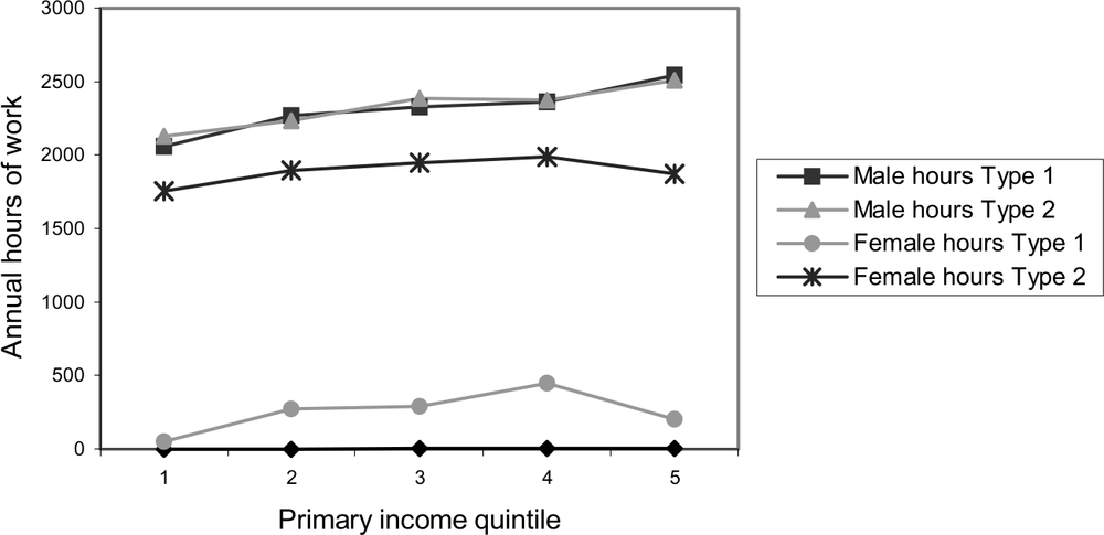
Note the relatively flat profile of primary income and earnings across quintiles 2 to 4. Within each quintile we can expect considerable variation in the second income, given the variation in employment status. Thus, a ranking defined on household income could well place a two-earner family working long hours for relatively low wages near the top quintile, due to the relatively flat profile of primary earnings across the middle quintiles. To show this more clearly, Table 4.2 presents data means for the incomes and labour supplies of two household groups of equal size, labelled Type 1 and Type 2, defined according to hours worked by the second earner. Type 1 households are those in which the second earner’s annual hours are below the median of the sample, and Type 2, those in which her hours are above the median.
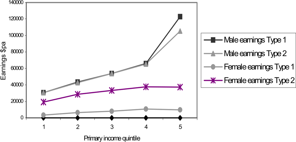
Figure 4.1 plots the primary and second hours profiles of the two household types, and Figure 4.2, the corresponding earnings profiles. The figures show graphically the very large gap between the average hours worked by the second earner of each type, and the correspondingly large gap between average second earnings, within each quintile. In contrast to second earners, the average primary earner in both household types works almost the same hours and has similar earnings, reflecting similar gross wage rates, except in the top quintile. It is evident from these profiles that little of the variation in female labour supply can be explained by primary wage rates, other than in the top quintile. Nor can it be explained adequately by demographics. The average number of 81dependent children in the Type 1 household is 2.0 and in the Type 2 household, 1.8.
Table 4.2 Quintile distribution by primary income and household type, 2006–07
| Quintile | 1 | 2 | 3 | 4 | 5 | All |
| Type 1 | ||||||
| Primary earnings $pa | 30 701 | 43 254 | 53 971 | 66 044 | 123 004 | 64 016 |
| Second earnings $pa | 3632 | 6542 | 8214 | 10 821 | 9755 | 19 159 |
| Primary market hours pa | 2058 | 2273 | 2326 | 2362 | 2544 | 2314 |
| Second market hours pa | 54 | 272 | 289 | 447 | 202 | 253 |
| Type 2 | ||||||
| Primary earnings $pa | 30 779 | 42 705 | 53 685 | 65 258 | 105 287 | 59 193 |
| Second earnings $pa | 19047 | 28494 | 33340 | 37655 | 37404 | 19159 |
| Primary market hours pa | 2132 | 2233 | 2269 | 2386 | 2508 | 2303 |
| Second market hours pa | 1754 | 1899 | 1949 | 1991 | 1873 | 1892 |
Figure 4.1 Family labour supplies by household type
82
Figure 4.2 Primary and second earnings by household type
We know from time use data that mothers who withdraw from market work after the first child spend long hours providing home child care and related services that they would otherwise need to buy-in, unless they have access to an ‘extended family’ arrangement (see Apps & Rees 2003, 2005). It is therefore essential to take account of home production in a measure of family welfare, in order to avoid the potential for large ranking errors as indicated by Table 4.2. For example, the average joint income of Type 2 families in quintile 2 is close to that of Type 1 families in quintile 4, yet much, if not all, of the net-of-tax second income of a Type 2 family may be spent on bought-in child care. Under these conditions, primary income is likely to be a far more reliable indicator of family living standards.
To highlight further the potential for ranking errors of this kind, Table 4.3 presents the earnings profiles of Type 1 and Type 2 families, for a ranking by household income. The table also reports the quintile distribution of the household types and the hours they work. Over half of the two-earner families in the bottom quintile of primary income are shifted to a higher quintile, and only 30 per cent remain in the bottom two quintiles. It is evident from the earnings and hours profiles that a ranking by household income is 83driven by the market hours of the second earner, rather than by wage rates, and therefore indirectly by the omission of implicit income from home production in household income as the ranking variable.
Table 4.3 Quintile distribution by household income and household type
| Quintile | 1 | 2 | 3 | 4 | 5 | All |
| Household income $pa | 37 057 | 57 841 | 74 557 | 94 332 | 15 3981 | 84 117 |
| % type 2 | 24.4 | 35.4 | 52.4 | 67.4 | 63.6 | 50.0 |
| Type 1 | ||||||
| Primary earnings $pa | 35 050 | 51 837 | 62 595 | 73 545 | 136 289 | 64 016 |
| Primary market hours pa | 2118 | 2260 | 2362 | 2389 | 2563 | 2314 |
| Second market hours pa | 56 | 226 | 430 | 471 | 286 | 253 |
| Type 2 | ||||||
| Primary earnings $pa | 29 135 | 37 866 | 45 841 | 58 968 | 92 885 | 59 193 |
| Primary market hours pa | 2132 | 2140 | 2284 | 2321 | 2452 | 2303 |
| Second market hours pa | 1620 | 1809 | 1917 | 1904 | 2004 | 1892 |
Family tax system
We now turn to the structure of effective tax rates on the incomes of family members, due to the interaction of personal income tax with the FTB system, the low income tax offset and Medicare Levy. Marginal and average rates on primary and second earnings are computed for the sample of ‘in-work’ families described in the previous section, and reported for a ranking defined on primary income as in Tables 4.1 and 4.2. Results are presented for two financial years, 2005–06 and 2006–07, to show the impact of changes in the 2006–07 Budget on the distribution of the family tax burden between primary and second earners. All incomes are indexed to the relevant financial year.
Table 4.4 reports, in row 1, the amount of tax the representative family in each quintile would pay if the second earner did not go out to work.10 The figures therefore give estimates of the average amount of tax families would pay on primary earnings and asset income in each quintile, if second earnings were zero. The overall
84average is $6648 per annum. The second row of the table reports the resulting average tax rate (ATR) on primary earnings and asset income. For the full sample, the ATR is 10.3 per cent. In other words, if all second earners withdrew from work, the overall average rate of tax on family income would be 10.3 per cent.
The third row of the table shows the tax on the income of the second earner, calculated for each record as the increment in the family’s tax burden due to her participation in the labour market. The overall average is $6266 pa. The final row gives the quintile profile of ATRs on second earnings. The overall ATR on the second income is 32.7 per cent, more than three times the ATR on primary earnings and asset income.
Table 4.4 Tax burdens on ‘in-work’ families, Budget 2006–07
| Quintile | 1 | 2 | 3 | 4 | 5 | All |
| All families – zero second earnings | ||||||
| Tax on income* $pa | -7401 | -1669 | 2929 | 8353 | 30 760 | 6648 |
| ATR % | -23.6 | -3.7 | 5.3 | 12.1 | 24.8 | 10.3 |
| Second earner | ||||||
| Tax on second earnings $pa | 3871 | 6314 | 6538 | 7197 | 7425 | 6266 |
| ATR on second earnings % | 34.6 | 35.4 | 31.8 | 30.8 | 32.3 | 32.7 |
* Primary earnings and asset income
These results indicate a very high degree of tax discrimination against the second earner. The average tax paid by the representative family in the sample is $12 914, the sum of the amount paid as a single-earner family, $6648, and the tax on second earnings, $6266. Thus, if all families had only one earner or, equivalently, if all second earners withdrew from work, average tax per family in the sample would fall from $12 914 pa to $6648 pa, that is, by 48.5 per cent. This dramatic fall is due to very high effective ATRs on second earnings. ATRs on primary income, and therefore on the incomes of single-earner families, are not only low on average but highly progressive. We have a negative income tax up to the second quintile, with those in quintile 1 receiving a net transfer that averages $7401 per annum. The ATR rises to 5.3 per cent in quintile 3, and to 24.8 per cent in quintile 5. This progressive taxation of primary incomes contrasts with the 85treatment of second earnings. Not only are ATRs on second earnings much higher, at over 30 per cent in all quintiles, the highest rate appears in quintile 2.
In an earlier paper I made the same calculation for the 2005–06 financial year using data for a sample of ‘in-work’ families from the earlier ABS 2002–03 SIH survey (Apps 2006b). The data for the sample of families selected for the present study, with incomes indexed to 2005–06, yield very similar figures. The results are presented in Table 4.5 in the same format as Table 4.4, showing in addition the changes in ATRs that flowed from the tax cuts introduced in the 2006–07 Budget.
The changes in ATRs reveal an especially interesting outcome of the 2006–07 Budget. The average family tax burden is computed as $14 415 for 2005–06, and found to fall to $8196 when calculated to exclude second earnings. This implies an effective average tax burden on the second earner of $6219 per annum, which is 43.4 per cent of the overall average family tax burden. Thus, the changes in the 2006–07 Budget increased the relative share of the burden on the second earner, from 43.4 per cent to over 48.5 per cent – a rise of over 5 percentage points.
Table 4.5 Tax burdens on ‘in-work’ families, Budget 2005–06
| Quintile | 1 | 2 | 3 | 4 | 5 | All |
| Panel 1 | ||||||
| Tax on income* $pa | -6303 | -92 | 4176 | 9560 | 33596 | 8196 |
| ATR% | -20.4 | -0.0 | 7.7 | 14.2 | 27.7 | 12.9 |
| 2006–07 change in ATR | -3.2 | -3.7 | -2.4 | -2.1 | -2.9 | -2.6 |
| Panel 2 | ||||||
| Tax on second earnings $pa | 4286 | 5940 | 6285 | 7175 | 7411 | 6219 |
| ATR% | 39.1 | 34 | 31.2 | 31.4 | 32.8 | 33.1 |
| 2006–07 change in ATR | -4.5 | 1.4 | 0.6 | -0.4 | -0.6 | -0.4 |
*Primary earnings and asset income
The higher relative burden on the second earner is a consequence of reducing the absolute burden on the primary earner, from an average of $8196 to $6648, while leaving the absolute burden on the second earner almost unchanged. The fall in the tax burden on primary earnings and asset income results in an overall reduction in 86the ATR on that income of 2.6 percentage points and, within each quintile, a consistent gain of over 2 percentage points. In contrast, the overall change in the ATR on second earnings is close to zero.11 There is a more substantial gain in quintile 1, of 4.5 percentage points, but this is then offset by losses in quintiles 2 and 3. In other words, the tax burden on second earners in these low-income quintiles actually increased in absolute value, due to the 2006–07 Budget changes.
The shift in the overall family tax burden to the second earner was achieved by combining personal income tax cuts for high income earners with tax-cuts for average income single-earner families through the expansion of the FTB system and tax cuts for very low income earners through the expansion of the low income tax offset. In the discussion to follow, the specific changes in these policy instruments in the 2006–07 Budget are explained in some detail, to show how they shift the tax burden to the second earner.
Table 4.6, Panel 1, lists the personal income tax rate schedules and thresholds for 2005–06 and 2006–07 financial years. The rise in the $21 600 threshold to $25 000 provides a tax cut of $510 per annum for an individual within the income range of $25 000 to $63 000 pa. The shift in the threshold of $63 000 to $75 000 for the 30 cents in the dollar rate gives an individual with an income of $75 000 an additional tax cut of $1440. For someone on an income of $150 000, these changes, together with the top threshold and rate changes, provide a total tax cut of $6200. Thus the personal income tax changes are very generous to the top, give little to the middle, and offer nothing to the bottom.
A tax cut for very low-income earners is provided by increasing the low income tax offset, from $235 to $600. The argument for an offset of this kind usually runs as follows. The aim of government is to reduce taxes on low and average income workers. One way of achieving this is to raise the zero-rated threshold to, say, $10 000. However, the resulting gain of $600 would go to all taxpayers above this threshold, including those on $150 000. And so, it is typically
87argued,12 a more effective use of government revenue is achieved by targeting the tax cut to the preferred low-income group through a tax offset.
Table 4.6 Income tax schedule and low income tax offset
Panel 1 Income tax schedule
| 2005–06: Taxable income | MTR* | 2006–07: Taxable income | MTR |
|
$0–$6000 $6001–$21 600 $21 601–$63 000 $63 001–$95 000 $95 000 + |
0.00 0.15 0.30 0.42 0.47 |
$0–$6000 $6001–$25 000 $25 001–$75 000 $75 001–$150 000 $150 000 + |
0.00 0.15 0.30 0.40 0.45 |
Panel 2 Income tax schedule and low income tax offset
| 2005–06: Taxable income | MTR | 2006–07 Taxable income | MTR |
|
$0–$7567 $7568–$21 600 $21 601–$27 475 $27 476–$63 000 $63 001–$95 000 $95 000 + |
0.00 0.15 0.34 0.30 0.42 0.47 |
$0–$10 000 $10 001–25 000 $25 001–$40 000 $40 001–$75 000 $75001–$150 000 $150 00 + |
0.00 0.15 0.34 0.30 0.40 0.45 |
*Marginal tax rate
Limiting the tax cut to those on low incomes is, however, clearly not the concern of the Howard government, given the large tax cuts at the top. To the contrary, the purpose of the offset is to deny those across a wide middle band of the earnings distribution, specifically from $40 000 to $63 0000, a tax cut of $600, while simultaneously providing much larger cuts at higher income levels. This is evident from Panel 2 of the table, which lists the effective MTR schedules in the two financial years incorporating the low income tax offset. In effect, the offset raises the MTR on incomes from $25 000 to $40 000 to 34 cents in the dollar, thereby introducing a ‘hump’ in the MTR profile across relatively low incomes. The offset is, in fact, an entirely redundant policy instrument. The same rate changes could have been announced simply, and more transparently, as the new MTR schedule shown in Panel 2. This would, of course, clarify the
88role of the offset as that of limiting to $510 the personal income tax cut for a parent earning from $40 000 and $63 000.
However, not every parent within this income range is denied a more substantial gain. As in previous budgets, single-earner families, and those in which the second earner’s income is more marginal, are compensated through the FTB system. It is only two-earner families with a more equal division of income who are left out in the cold. The increase in the lower income threshold for the withdrawal of FTB Part A from $34 290 ($33 361 in 2005–06) to $40 000 provides a tax cut of $1142 for each child up to the income level at which this gain is the remaining amount to be withdrawn. For the two-earner family in which the second earner has a more significant workforce attachment, the gain can be entirely lost at relatively low wage levels because FTB Part A is withdrawn on joint income.
The following tables illustrate the impact of the system in 2005–06, and of the changes introduced in the 2006–07 Budget, for the family with three children under 12, including one under 5 years, and with income from earnings only. Table 4.7 first of all lists effective marginal tax rate rates and thresholds for the single-earner family, for the two financial years. The rates are calculated to include income taxes, the low income tax offset, the Medicare Levy and FTBs Part A and Part B. Since second earnings are zero, the family is eligible for the full amount of FTB Part B, that is, for $3372.60 in 2005–06 and $3467.50 in 2006–07.
The MTR profiles in both years exhibits a much stronger ‘hump’ or inverted U-shape, due to the withdrawal of FTB Part A at 20 cents in the dollar from $33 362 in 2005–06 and $40 000 in 2006–07, and the withdrawal of the Medicare Levy low income exemption. The second hump in the profiles further along the distribution is due to the withdrawal of the base rate of FTB Part A at 30 cents in the dollar. Since both FTB Part A and the Medicare Levy exemption are withdrawn on joint income, a second earner going out to work within the income range of the first ‘hump’ will face an effective tax rate that includes the withdrawal rates of both. In addition, she will lose an extra 20 cents in the dollar due to the withdrawal of FTB Part B. The end result is an income tax system that very closely approximates one of joint taxation across much of the distribution of family income, but with a difference. Under a conventional joint 89tax (or income splitting) system, the MTR schedule is typically progressive. Australian families face an inverted U-shaped schedule.
Table 4.7 Effective marginal tax rates schedules for the singleearner family
| 2005–06 | 2006–07 | ||
| Taxable income | MTR | Taxable income | MTR |
|
$0–$7567 $7568–$21 600 $21 601–$27 475 $27 476–$33 361 $33 362–$34 226 $34 227–$37 001 $37 002–$63 000 $63 001–$69 715 $69 716–$93 074 $93 075–$95 000 $95 001–$110 850 $110 850+ |
0.00 0.15 0.34 0.30 0.50 0.70 0.515 0.635 0.435 0.735 0.785 0.485 |
$0–$10 000 $10 001–$25 000 $25 001–$35 048 $35 049–$40 000 $40 001–$41 232 $41 233–$75 000 $75 001–$77 336 $77 337–$95 631 $95 632–$113 911 $113 912–$150 000 $150 000 + |
0.00 0.15 0.34 0.44 0.60 0.515 0.615 0.415 0.715 0.415 0.465 |
Because the 2006–07 Budget reduces tax burdens for the average income single-earner family by raising the threshold for the withdrawal of FTB Part A and lowering the rate of withdrawal for the Medicare Levy exemption, the hump in the MTR profile shifts along the distribution, and is also extended, as shown in Table 4.7. The Budget changes therefore have the effect of bringing more families on average incomes into the net of a system of joint taxation with an inverted U-shaped MTR schedule. The second earner can face especially high effective MTRs and ATRs as she increases her hours of work if the primary earner of the family falls within the income range of the first hump in the MTR profile. Table 4.8 gives, as an example, the MTRs and ATRs on the second earnings of a family in which primary income is $40 000 pa in both financial years.
In 2005–06 the second earner lost almost half her income at around $20 000. While the 2006–07 Budget reduced losses for second earners at lower income levels, it raised rates as her income approached that of the primary earner. At $40 000, for example, the second earner’s MTR and ATR are, in fact, higher in 2006–07. When both parents earn $40 000 per annum, a figure that is well 90below average earnings, the second earner loses 47.5 per cent of her wages, which is more than she would have lost in the previous year. This is because the 2006–07 Budget changes were designed to exclude the family with more equal partner incomes from a gain from the rise in the FTB Part A lower income threshold to $40 000, and from a personal tax cut above $510 for each parent, by completely withdrawing the low income offset at $40 000. These measures not only have the effect of shifting the share of the family tax burden towards the second earner, they also shift the overall tax burden towards two-earner families in which each parent’s income ranges from around $40 000 to $63 000. Thus, while the new discrimination impacts directly on the second earner, its indirect effect is upon families in which both parents work full-time to earn similar but relatively low and average wages.
Table 4.8 Second earner’s effective marginal and average tax rates*
| 2005–06 | 2006–07 | ||||
| Second earner’s taxable income |
MTR | ATR | Second earner’s taxable income |
MTR | ATR |
|
$0–$4088 $4089–$7567 $7568–$20 951 $20 952–$21 000 $21 001–$27 475 $27 476–$29 715 $29 716–$40 000 |
0.215 0.415 0.565 0.365 0.555 0.515 0.315 |
0.215 0.307 0.472 0.469 0.487 0.488 0.444 |
$0–$1232 $1233–$4234 $4235–$10 000 $10 001–$21 572 $21 573–$25 000 $25 001–$37 337 $37 338–$40 000 |
0.30 0.215 0.415 0.565 0.365 0.555 0.355 |
0.280 0.240 0.341 0.461 0.448 0.483 0.475 |
* Primary earner income = $40 000 pa
To give an indication of the distributional limitations of the federal government’s new tax system in 2006–07, Table 4.9 translates family tax burdens into ‘hours worked to pay tax’, or the ‘hours of work equivalent’ of the family’s tax, for Type 1 and Type 2 households, by quintiles of primary income. The first row for each type reports the average tax burden on families in each quintile, and the second row, hours worked to pay tax.
In quintile 3, the average tax burden for the Type 2 household is equivalent to 764 hours of work for the government per year. This is more than the hours worked to pay tax by the average Type 1 household in quintile 5 on a much higher income. The Type 2 91household in quintile 2 works an average of 574 hours for the government. This is some 50 per cent higher than the hours reported for a Type 1 household in quintile 4, and is approaching the number of hours worked for the government by the Type 1 household in quintile 5, on a very much higher primary income.
Table 4.9 Hours worked to pay tax, by primary income and household type, 2006–07
| Quintile | 1 | 2 | 3 | 4 | 5 | All |
| Type 1 | ||||||
| Total tax $pa | -6956 | 43 | 4412 | 10991 | 37 308 | 9456 |
| Hours worked to pay tax | - | - | 155 | 394 | 687 | - |
| Type 2 | ||||||
| Total tax $pa | 38 | 9010 | 14 720 | 20 760 | 39 141 | 16 545 |
| Hours worked to pay tax pa | - | 574 | 764 | 925 | 1177 | - |
Taxes on second earners and their families at these levels, together with a lack of access to affordable, high quality child care, can be expected to have strong negative effects on female labour supply, not only during the child rearing years but throughout the life cycle (see Shaw 1994). This is evident from lifecycle time allocation profiles for selected OECD countries reported in Apps (2006a).
Conclusion
In this chapter I have argued that the Australian family tax system is fundamentally flawed as a result of policy changes that have transformed it from a progressive individual income tax system to one much more closely resembling joint taxation. These policies constitute what I have elsewhere labelled the ‘new discrimination’. The problem lies not in the level of family benefits, but in the effective marginal tax rate schedule created by the withdrawal of benefits on household income and the income of the second earner. The introduction of this new system over successive budgets has shifted the tax burden from single-earner to two-earner couples in a way that is bad for both efficiency and equity.92
Policies that raise marginal rates on the second income tax more heavily the partner with the more elastic labour supply, in contradiction of the standard principle for minimising the deadweight efficiency loss from taxation. The resulting tax rate structure seriously inhibits the reallocation of female time from the household to the market during a period of declining fertility and therefore of falling demand for domestic labour.13
Imposing high average tax rates on the second income also ignores the fact that of two households with the same total household income, where one has the second earner working entirely in the market, the other entirely in the household, the latter will have a significantly higher standard of living because of its higher level of output of household goods and services.
Large family benefits can be justified as a response to market failure. Children, or their parents as their agents, cannot borrow on capital markets against their future incomes to finance their current consumption and investment in human capital, or obtain cover in insurance markets for the risks they face. In the absence of public support, not by financial transfers but by a publicly funded school system, there would be underinvestment in the next generation. It does not seem to be appreciated that a similar argument applies to child care, a badly neglected sector in Australia. A high quality, affordable, publicly provided child care system would more than repay itself in expanded female labour supply and the likely increase in fertility that would result from making it more feasible for women to combine a career with having children.
Acknowledgement
I would like to thank Margi Wood for her contribution to programming and data management for the study. The research was supported by an Australian Research Council DP Grant.
93
References
Apps, PF 2006a, Female labour supply, taxation, and the new discrimination, Presidential Address, XX Annual Conference of the European Society for Population Economics, Verona, June 22–24.
Apps, PF 2006b, Family taxation: an unfair and inefficient system, Australian Review of Public Affairs, vol. 7, pp. 77–101.
Apps, PF & Rees, R 1999, ‘Individual vs. joint taxation in models with household production, Journal of Political Economy, vol. 107, pp. 393–403.
Apps, PF & Rees, R 2003, ‘Life Cycle Time Allocation and Saving in an Imperfect Capital Market’, NBER Summer Institute Session on: Aggregate Implications of Microeconomic Consumption Behavior, Boston, July 21–25, available as IZA DP 1036: www.iza.org.
Apps, PF & Rees, R 2005, ‘Gender, time use, and public policy over the life cycle’, Oxford Review of Economic Policy, vol. 21, pp. 439–61.
Australian Bureau of Statistics 2006, Household Expenditure Survey and Survey of Income and Housing – Confidentialised Unit Record Files, Australia 2003–04, technical paper 6540.0.00.001., ABS, Canberra.
Boskin, MJ & Sheshinski E 1983, ‘Optimal tax treatment of the family’, Journal of Public Economics, vol. 20, pp. 281–297.
Eissa, N & Hoynes, H 2005, ‘Behavioral responses to taxes: lessons from the EITC and labor supply’, paper for the Tax Policy and the Economy conference, 15 September, Washington DC.
Ellwood, DT & Liebman, JB 2000, The middle class parent penalty: child benefits in the US tax code, working paper 8031, NBER, Cambridge, Mass.94
Feldstein, M & Feenberg, DR 1996, ‘The taxation of two-earner families’, in M Feldstein and JM Poterba (eds), Empirical foundations of household taxation, NBER Project Report, University of Chicago Press, Chicago.
Jaumotte, F 2003, Female labour force participation: past trends and main determinants in OECD countries, working paper 376, Economics Department, OECD, Paris.
Organisation for Economic Co-operation and Development 2006, Taxing Wages 2004–2005, OECD, Paris.
Shaw, K 1994, ‘The persistence of female labor supply: empirical evidence and implications’, Journal of Human Resources, vol. 29, pp. 348–78.
1 See Ellwood and Liebman (2000) and Eissa and Hoynes (2005) for studies that identify the changes in effective tax rates introduced by these programs.
2 See Tables III.5c, p.92, III.6c, p.95, and III.7c, p.98.
3 For a life cycle analysis that shows this using Australian data see Apps and Rees (2003).
4 The argument against this proposition implies two key assumptions: that a parent working full-time at home caring for young children is unproductive and her life of leisure is supported by an altruistic hand-out from her husband equal to half his income.
5 See Jaumotte (2003) for estimates of the ‘tax wedge’ for OECD countries, calculated as the ratio of the effective tax on the second earner’s income and the tax she would face as a single individual with the same income.
6 As does high-cost, for profit, child care in an imperfect capital market (see Apps and Rees, 2003).
7 The Boskin and Sheshinski analysis is an application of the Ramsey pricing rule: for efficiency, effective tax rates should be related inversely to (compensated) wage/price elasticities. For a more recent empirical analysis which comes to a similar conclusion, see Feldstein and Feenberg (1996).
8 Of male partners in all two-parent families, 83.6 per cent are in full-time work, 6.7 per cent are in part-time work and 2.5 per cent are unemployed. Of married mothers in the same sample, 27.9 per cent are in full-time employment, 37.6 per cent are in part-time work and 2.3 per cent report being unemployed.
9 Note that asset income is given by the difference between income and earnings and, on average, contributes little to family incomes except in the top quintile.
10 All figures are weighted means.
11 Note that even though the tax on second earnings rose slightly in 2006–07, the increase was not in line with the indexed rise in earnings. This explains the fall in the overall ATR of 0.4 of a percentage point.
12 The argument, of course, reflects a fundamental misunderstanding of the role of the different policy instruments in setting the tax rate structure, as discussed in section 2 of Apps (2006b).
13 For further discussion, and comparisons with the tax systems of the USA, UK and Sweden, see Apps (2006a).